Chapter 3: Even more customizations in ggplot2

In this chapter, we will learn how to change the theme settings of a graph in {ggplot2} The theme of a graph consists of non-data components present in your graph. This includes the different labels of the graph, fonts used, colour of axes, the background of the graph etc. By changing the theme we would not be changing or transforming how the data will look in the graph. Instead, we would only change the visual appearances in the graph and by doing so we can make it more aesthetically pleasing. Furthermore, we will see a few popular packages featuring ready to use themes. We will also learn about colour palettes and will see different packages associated with them.

1 Complete themes

The {ggplot2} package features ready to use themes called ‘complete themes’. So before we begin customizing themes, let us plot a few graphs and see how these themes look like. For the plots, I have used the BirdNest dataset from the {Stat2Data} package in R. The BirdNest dataset contains nest and species characteristics of North American passerines. The data was collected by Amy R. Moore, as a student at Grinnell College in 1999.

• Getting the BirdNest dataset and viewing how the dataset is structured.

install.packages("Stat2Data") # for installing Stat2Data package
install.packages("ggplot2") # for installing ggplot2 package

# load the packages
library(Stat2Data)
library(ggplot2)

data("BirdNest") # loading the BirdNest dataset
str(BirdNest) # for viewing structure of the dataset

So we have plenty of variables to play with. The tabs shown below are named according to the theme used in the plots.

theme_gray()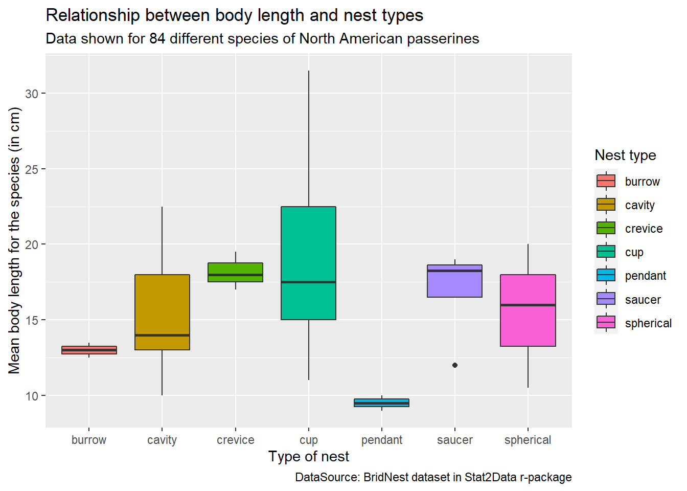

Show the code

library(Stat2Data)
library(ggplot2)
data("BirdNest")

ggplot(BirdNest, aes(Nesttype, Length, fill = Nesttype)) + geom_boxplot() + 
  labs(x= "Type of nest", y= "Mean body length for the species (in cm)",
       fill= "Nest type", title= "Relationship between body length and nest types",
       subtitle = "Data shown for 84 different species of North American passerines",
       caption= "DataSource: BridNest dataset in Stat2Data r-package") +
  theme_gray()

theme_bw()

Show the code

library(Stat2Data)
library(ggplot2)
data("BirdNest")

ggplot(BirdNest, aes(Nesttype, Length, fill = Nesttype)) + geom_boxplot() + 
  labs(x= "Type of nest", y= "Mean body length for the species (in cm)",
       fill= "Nest type", title= "Relationship between body length and nest types",
       subtitle = "Data shown for 84 different species of North American passerines",
       caption= "DataSource: BridNest dataset in Stat2Data r-package") +
  theme_bw()

theme_linedraw()

Show the code

library(Stat2Data)
library(ggplot2)
data("BirdNest")

ggplot(BirdNest, aes(Nesttype, Length, fill = Nesttype)) + geom_boxplot() + 
  labs(x= "Type of nest", y= "Mean body length for the species (in cm)",
       fill= "Nest type", title= "Relationship between body length and nest types",
       subtitle = "Data shown for 84 different species of North American passerines",
       caption= "DataSource: BridNest dataset in Stat2Data r-package") +
  theme_linedraw()

theme_light()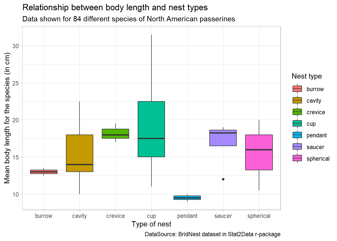

Show the code

library(Stat2Data)
library(ggplot2)
data("BirdNest")

ggplot(BirdNest, aes(Nesttype, Length, fill = Nesttype)) + geom_boxplot() + 
  labs(x= "Type of nest", y= "Mean body length for the species (in cm)",
       fill= "Nest type", title= "Relationship between body length and nest types",
       subtitle = "Data shown for 84 different species of North American passerines",
       caption= "DataSource: BridNest dataset in Stat2Data r-package") +
  theme_light()

theme_dark()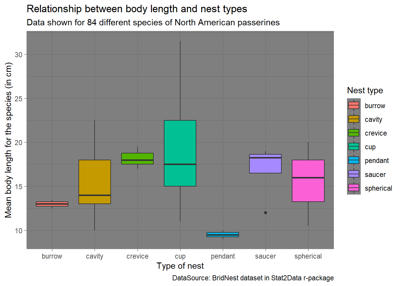

Show the code

library(Stat2Data)
library(ggplot2)
data("BirdNest")

ggplot(BirdNest, aes(Nesttype, Length, fill = Nesttype)) + geom_boxplot() + 
  labs(x= "Type of nest", y= "Mean body length for the species (in cm)",
       fill= "Nest type", title= "Relationship between body length and nest types",
       subtitle = "Data shown for 84 different species of North American passerines",
       caption= "DataSource: BridNest dataset in Stat2Data r-package") +
  theme_dark()

theme_minimal()

Show the code

library(Stat2Data)
library(ggplot2)
data("BirdNest")

ggplot(BirdNest, aes(Nesttype, Length, fill = Nesttype)) + geom_boxplot() + 
  labs(x= "Type of nest", y= "Mean body length for the species (in cm)",
       fill= "Nest type", title= "Relationship between body length and nest types",
       subtitle = "Data shown for 84 different species of North American passerines",
       caption= "DataSource: BridNest dataset in Stat2Data r-package") +
  theme_minimal()

theme_classic()

Show the code

library(Stat2Data)
library(ggplot2)
data("BirdNest")

ggplot(BirdNest, aes(Nesttype, Length, fill = Nesttype)) + geom_boxplot() + 
  labs(x= "Type of nest", y= "Mean body length for the species (in cm)",
       fill= "Nest type", title= "Relationship between body length and nest types",
       subtitle = "Data shown for 84 different species of North American passerines",
       caption= "DataSource: BridNest dataset in Stat2Data r-package") +
  theme_classic()

theme_void()

Show the code

library(Stat2Data)
library(ggplot2)
data("BirdNest")

ggplot(BirdNest, aes(Nesttype, Length, fill = Nesttype)) + geom_boxplot() + 
  labs(x= "Type of nest", y= "Mean body length for the species (in cm)",
       fill= "Nest type", title= "Relationship between body length and nest types",
       subtitle = "Data shown for 84 different species of North American passerines",
       caption= "DataSource: BridNest dataset in Stat2Data r-package") +
  theme_void()

2 Themes from ggthemes package

If you want even more pre-built themes then you can try the {ggthemes} package. This package was developed by Dr. Jeffrey B. Arnold.

# install and load ggthemes package
install.packages("ggthemes")
library(ggthemes)

The tabs shown below are named after the themes present in {ggthemes} package.

theme_base()

Show the code

library(Stat2Data)
library(ggthemes)
data("BirdNest")

ggplot(BirdNest, aes(Nesttype, Length, fill = Nesttype)) + geom_boxplot() + 
  labs(x= "Type of nest", y= "Mean body length for the species (in cm)",
       fill= "Nest type", title= "Relationship between body length and nest types",
       subtitle = "Data shown for 84 different species of North American passerines",
       caption= "DataSource: BridNest dataset in Stat2Data r-package") +
  theme_base()

theme_calc()

Show the code

library(Stat2Data)
library(ggthemes)
data("BirdNest")

ggplot(BirdNest, aes(Nesttype, Length, fill = Nesttype)) + geom_boxplot() + 
  labs(x= "Type of nest", y= "Mean body length for the species (in cm)",
       fill= "Nest type", title= "Relationship between body length and nest types",
       subtitle = "Data shown for 84 different species of North American passerines",
       caption= "DataSource: BridNest dataset in Stat2Data r-package") +
  theme_calc()

theme_clean()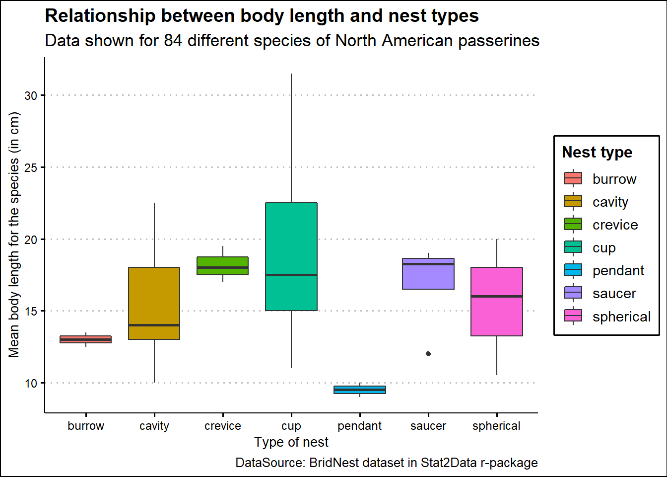

Show the code

library(Stat2Data)
library(ggthemes)
data("BirdNest")

ggplot(BirdNest, aes(Nesttype, Length, fill = Nesttype)) + geom_boxplot() + 
  labs(x= "Type of nest", y= "Mean body length for the species (in cm)",
       fill= "Nest type", title= "Relationship between body length and nest types",
       subtitle = "Data shown for 84 different species of North American passerines",
       caption= "DataSource: BridNest dataset in Stat2Data r-package") +
  theme_clean()

theme_economist()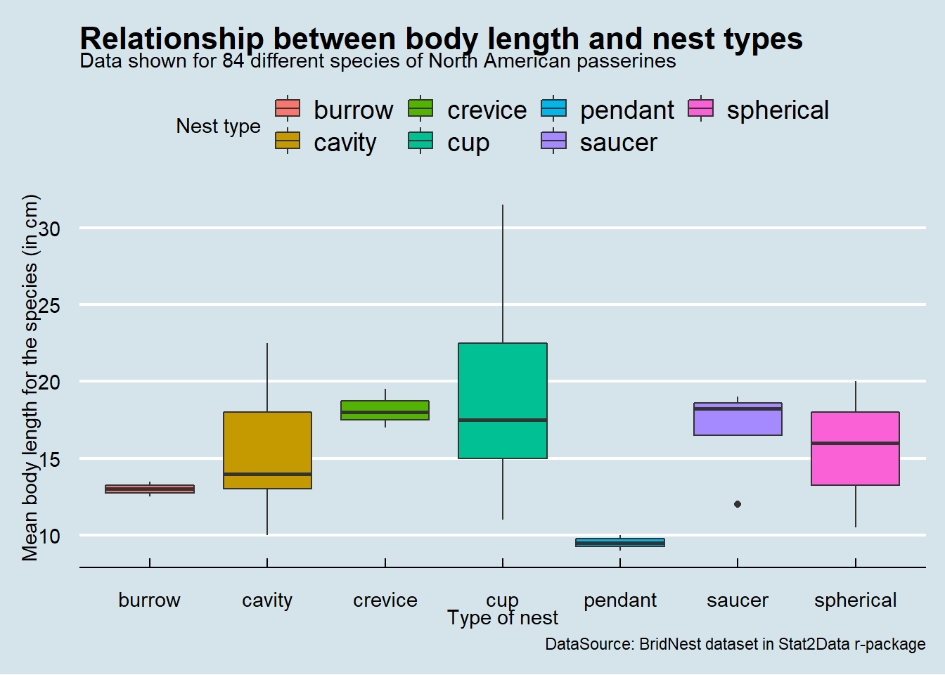

Show the code

library(Stat2Data)
library(ggthemes)
data("BirdNest")

ggplot(BirdNest, aes(Nesttype, Length, fill = Nesttype)) + geom_boxplot() + 
  labs(x= "Type of nest", y= "Mean body length for the species (in cm)",
       fill= "Nest type", title= "Relationship between body length and nest types",
       subtitle = "Data shown for 84 different species of North American passerines",
       caption= "DataSource: BridNest dataset in Stat2Data r-package") +
  theme_economist()

theme_excel()

Show the code

library(Stat2Data)
library(ggthemes)
data("BirdNest")

ggplot(BirdNest, aes(Nesttype, Length, fill = Nesttype)) + geom_boxplot() + 
  labs(x= "Type of nest", y= "Mean body length for the species (in cm)",
       fill= "Nest type", title= "Relationship between body length and nest types",
       subtitle = "Data shown for 84 different species of North American passerines",
       caption= "DataSource: BridNest dataset in Stat2Data r-package") +
  theme_excel()

theme_excel_new()

Show the code

library(Stat2Data)
library(ggthemes)
data("BirdNest")

ggplot(BirdNest, aes(Nesttype, Length, fill = Nesttype)) + geom_boxplot() + 
  labs(x= "Type of nest", y= "Mean body length for the species (in cm)",
       fill= "Nest type", title= "Relationship between body length and nest types",
       subtitle = "Data shown for 84 different species of North American passerines",
       caption= "DataSource: BridNest dataset in Stat2Data r-package") +
  theme_excel_new()

theme_few()

Show the code

library(Stat2Data)
library(ggthemes)
data("BirdNest")

ggplot(BirdNest, aes(Nesttype, Length, fill = Nesttype)) + geom_boxplot() + 
  labs(x= "Type of nest", y= "Mean body length for the species (in cm)",
       fill= "Nest type", title= "Relationship between body length and nest types",
       subtitle = "Data shown for 84 different species of North American passerines",
       caption= "DataSource: BridNest dataset in Stat2Data r-package") +
  theme_few()

theme_fivethirtyeight()

Show the code

library(Stat2Data)
library(ggthemes)
data("BirdNest")

ggplot(BirdNest, aes(Nesttype, Length, fill = Nesttype)) + geom_boxplot() + 
  labs(x= "Type of nest", y= "Mean body length for the species (in cm)",
       fill= "Nest type", title= "Relationship between body length and nest types",
       subtitle = "Data shown for 84 different species of North American passerines",
       caption= "DataSource: BridNest dataset in Stat2Data r-package") +
  theme_fivethirtyeight()

theme_foundation()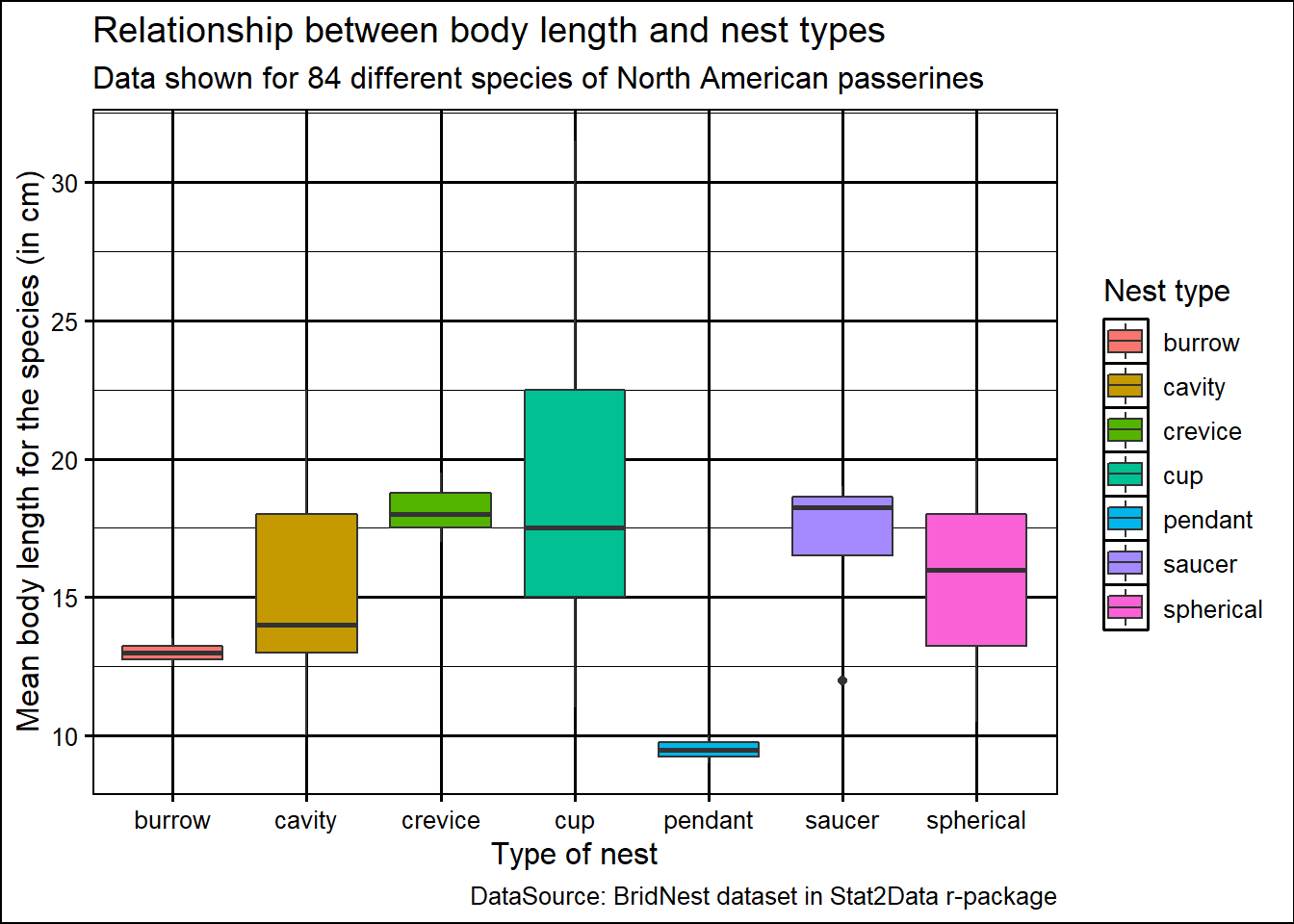

Show the code

library(Stat2Data)
library(ggthemes)
data("BirdNest")

ggplot(BirdNest, aes(Nesttype, Length, fill = Nesttype)) + geom_boxplot() + 
  labs(x= "Type of nest", y= "Mean body length for the species (in cm)",
       fill= "Nest type", title= "Relationship between body length and nest types",
       subtitle = "Data shown for 84 different species of North American passerines",
       caption= "DataSource: BridNest dataset in Stat2Data r-package") +
  theme_foundation()

theme_gdocs()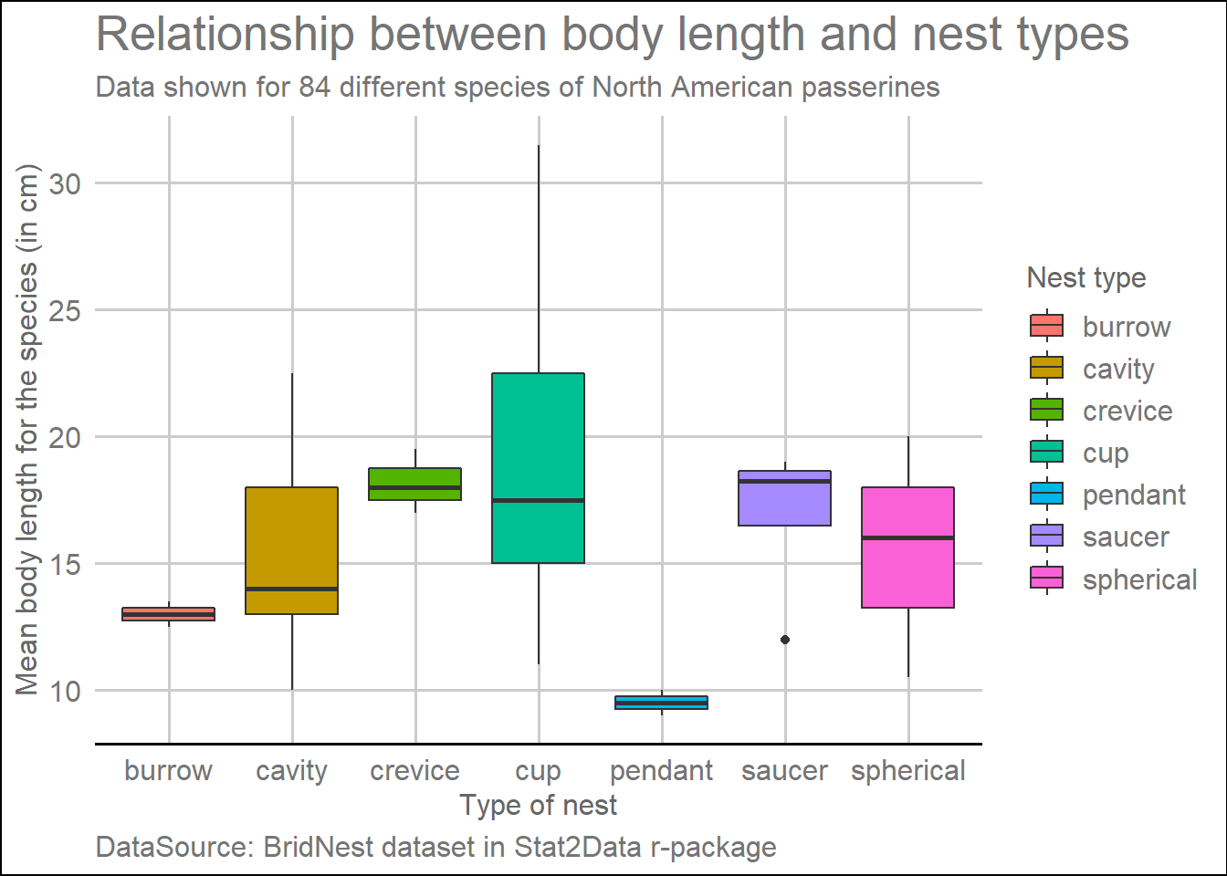

Show the code

library(Stat2Data)
library(ggthemes)
data("BirdNest")

ggplot(BirdNest, aes(Nesttype, Length, fill = Nesttype)) + geom_boxplot() + 
  labs(x= "Type of nest", y= "Mean body length for the species (in cm)",
       fill= "Nest type", title= "Relationship between body length and nest types",
       subtitle = "Data shown for 84 different species of North American passerines",
       caption= "DataSource: BridNest dataset in Stat2Data r-package") +
  theme_gdocs()

theme_hc()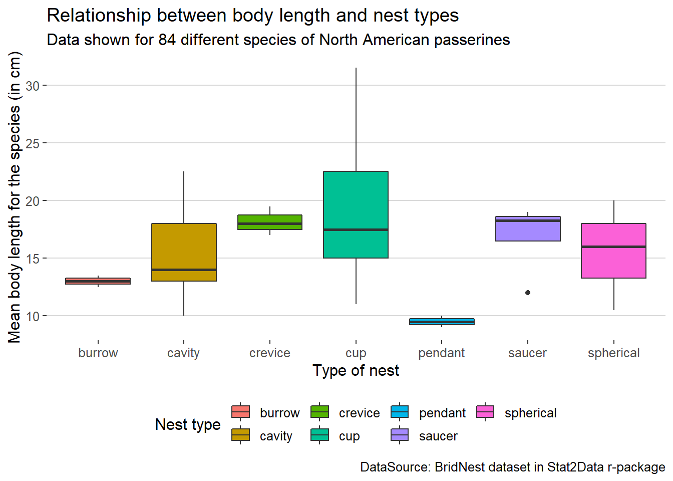

Show the code

library(Stat2Data)
library(ggthemes)
data("BirdNest")

ggplot(BirdNest, aes(Nesttype, Length, fill = Nesttype)) + geom_boxplot() + 
  labs(x= "Type of nest", y= "Mean body length for the species (in cm)",
       fill= "Nest type", title= "Relationship between body length and nest types",
       subtitle = "Data shown for 84 different species of North American passerines",
       caption= "DataSource: BridNest dataset in Stat2Data r-package") +
  theme_hc()

theme_igray()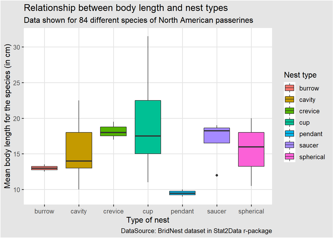

Show the code

library(Stat2Data)
library(ggthemes)
data("BirdNest")

ggplot(BirdNest, aes(Nesttype, Length, fill = Nesttype)) + geom_boxplot() + 
  labs(x= "Type of nest", y= "Mean body length for the species (in cm)",
       fill= "Nest type", title= "Relationship between body length and nest types",
       subtitle = "Data shown for 84 different species of North American passerines",
       caption= "DataSource: BridNest dataset in Stat2Data r-package") +
  theme_igray()

theme_map()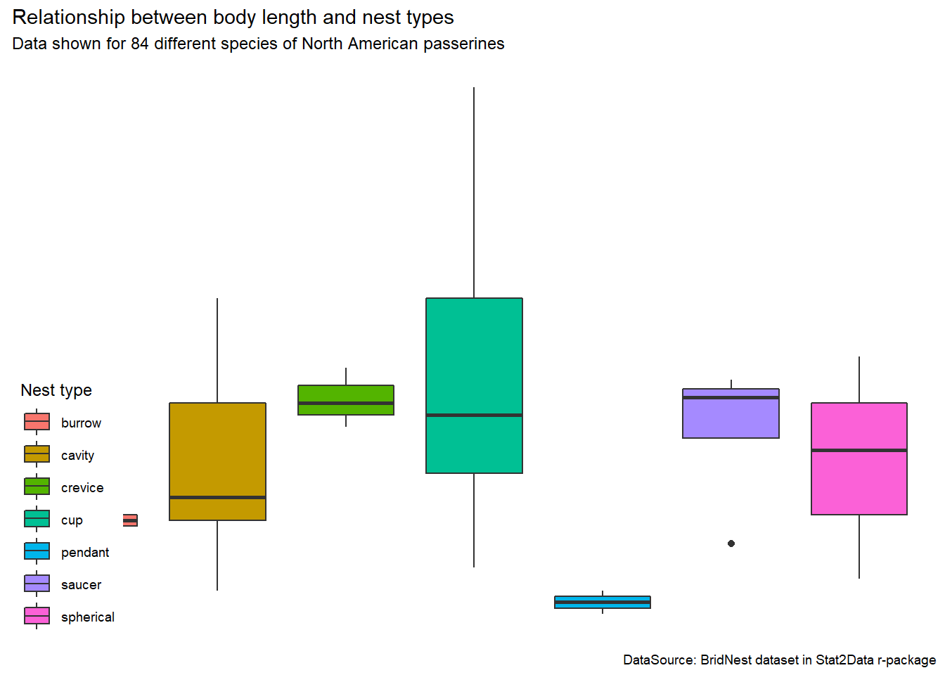

Show the code

library(Stat2Data)
library(ggthemes)
data("BirdNest")

ggplot(BirdNest, aes(Nesttype, Length, fill = Nesttype)) + geom_boxplot() + 
  labs(x= "Type of nest", y= "Mean body length for the species (in cm)",
       fill= "Nest type", title= "Relationship between body length and nest types",
       subtitle = "Data shown for 84 different species of North American passerines",
       caption= "DataSource: BridNest dataset in Stat2Data r-package") +
  theme_map()

theme_pander()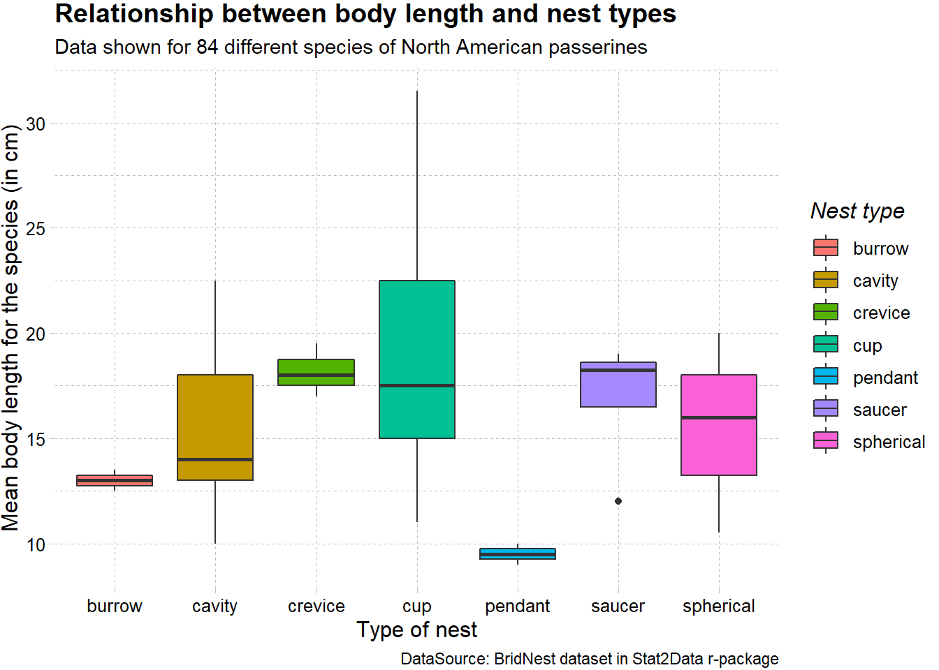

Show the code

library(Stat2Data)
library(ggthemes)
data("BirdNest")

ggplot(BirdNest, aes(Nesttype, Length, fill = Nesttype)) + geom_boxplot() + 
  labs(x= "Type of nest", y= "Mean body length for the species (in cm)",
       fill= "Nest type", title= "Relationship between body length and nest types",
       subtitle = "Data shown for 84 different species of North American passerines",
       caption= "DataSource: BridNest dataset in Stat2Data r-package") +
  theme_pander()

theme_par()

Show the code

library(Stat2Data)
library(ggthemes)
data("BirdNest")

ggplot(BirdNest, aes(Nesttype, Length, fill = Nesttype)) + geom_boxplot() + 
  labs(x= "Type of nest", y= "Mean body length for the species (in cm)",
       fill= "Nest type", title= "Relationship between body length and nest types",
       subtitle = "Data shown for 84 different species of North American passerines",
       caption= "DataSource: BridNest dataset in Stat2Data r-package") +
  theme_par()

theme_solarized()

Show the code

library(Stat2Data)
library(ggthemes)
data("BirdNest")

ggplot(BirdNest, aes(Nesttype, Length, fill = Nesttype)) + geom_boxplot() + 
  labs(x= "Type of nest", y= "Mean body length for the species (in cm)",
       fill= "Nest type", title= "Relationship between body length and nest types",
       subtitle = "Data shown for 84 different species of North American passerines",
       caption= "DataSource: BridNest dataset in Stat2Data r-package") +
  theme_solarized()

theme_solid()

Show the code

library(Stat2Data)
library(ggthemes)
data("BirdNest")

ggplot(BirdNest, aes(Nesttype, Length, fill = Nesttype)) + geom_boxplot() + 
  labs(x= "Type of nest", y= "Mean body length for the species (in cm)",
       fill= "Nest type", title= "Relationship between body length and nest types",
       subtitle = "Data shown for 84 different species of North American passerines",
       caption= "DataSource: BridNest dataset in Stat2Data r-package") +
  theme_solid()

theme_stata()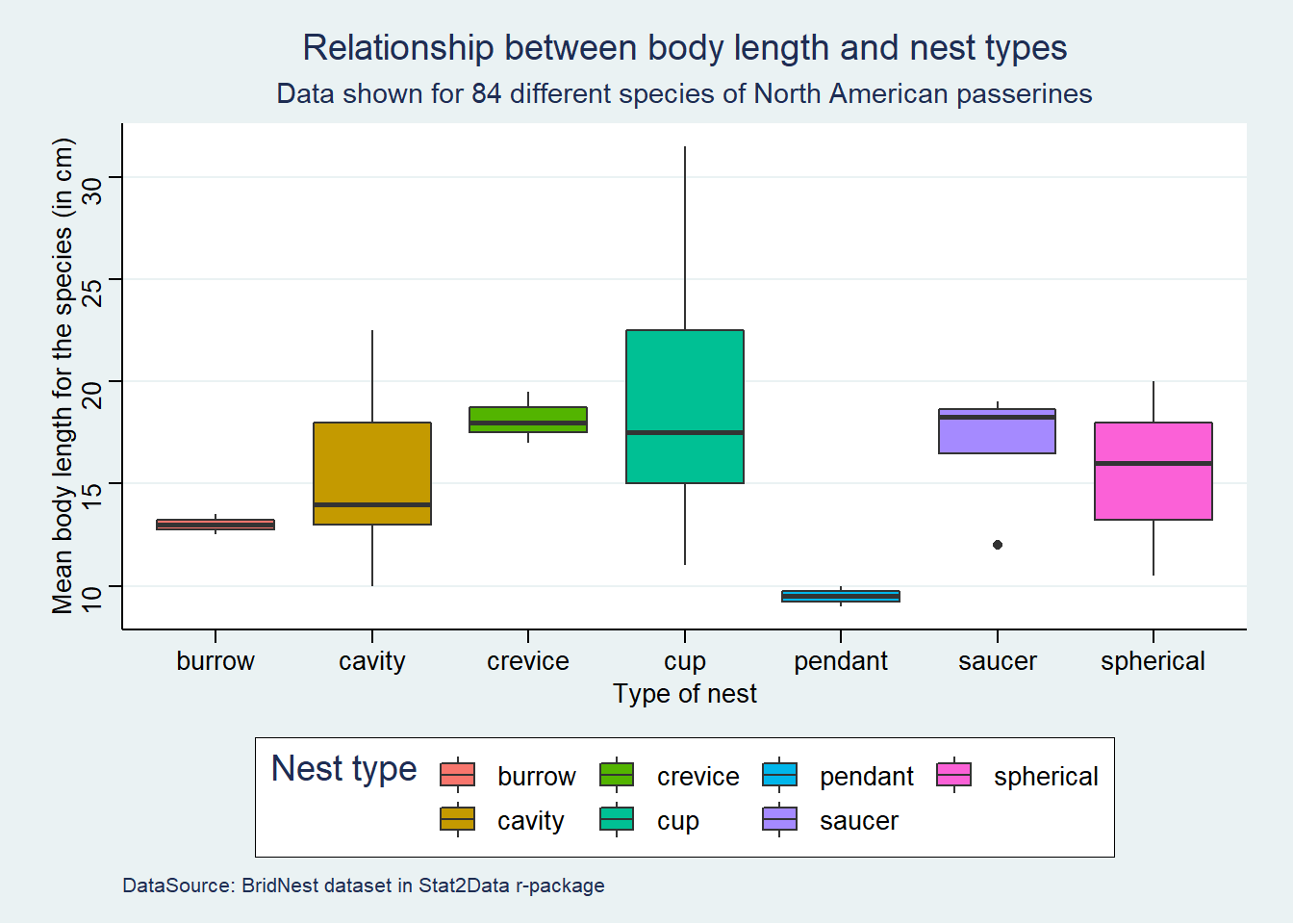

Show the code

library(Stat2Data)
library(ggthemes)
data("BirdNest")

ggplot(BirdNest, aes(Nesttype, Length, fill = Nesttype)) + geom_boxplot() + 
  labs(x= "Type of nest", y= "Mean body length for the species (in cm)",
       fill= "Nest type", title= "Relationship between body length and nest types",
       subtitle = "Data shown for 84 different species of North American passerines",
       caption= "DataSource: BridNest dataset in Stat2Data r-package") +
  theme_stata()

theme_tufte()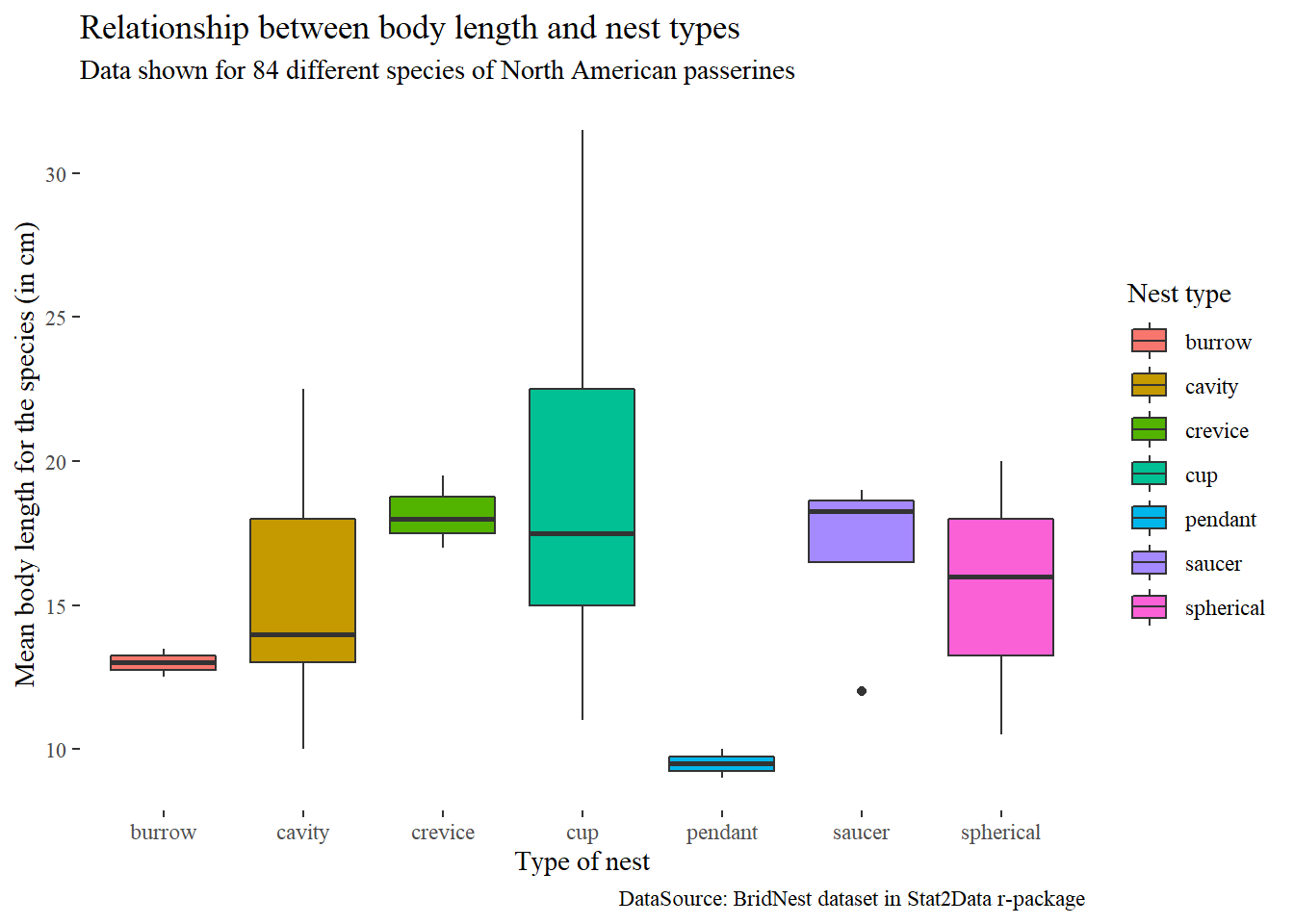

Show the code

library(Stat2Data)
library(ggthemes)
data("BirdNest")

ggplot(BirdNest, aes(Nesttype, Length, fill = Nesttype)) + geom_boxplot() + 
  labs(x= "Type of nest", y= "Mean body length for the species (in cm)",
       fill= "Nest type", title= "Relationship between body length and nest types",
       subtitle = "Data shown for 84 different species of North American passerines",
       caption= "DataSource: BridNest dataset in Stat2Data r-package") +
  theme_tufte()

theme_wsj()

Show the code

library(Stat2Data)
library(ggthemes)
data("BirdNest")

ggplot(BirdNest, aes(Nesttype, Length, fill = Nesttype)) + geom_boxplot() + 
  labs(x= "Type of nest", y= "Mean body length for the species (in cm)",
       fill= "Nest type", title= "Relationship between body length and nest types",
       subtitle = "Data shown for 84 different species of North American passerines",
       caption= "DataSource: BridNest dataset in Stat2Data r-package") +
  theme_wsj()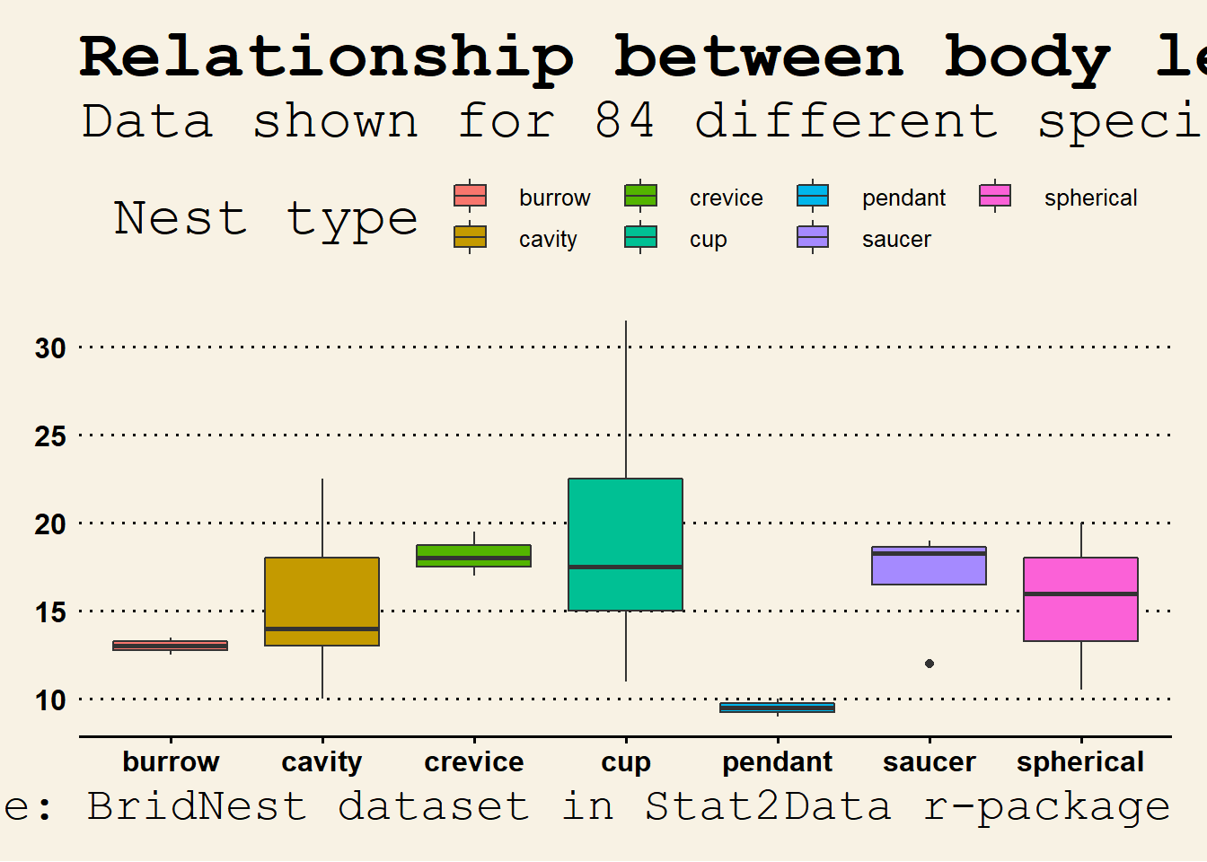

3 Changing colour palettes in ggplot2

Apart from ready to use themes, there are also ready to use colour palettes which we can use. A colour palette contains a set of pre-defined colours which will be applied to the different geometries present in a graph.

Choosing a good colour palette is important as it helps us to represent data in a better way and at the same time, it also makes the graph easier to read for people with colour blindness. Let us see a few popular colour palette packages used in R.

3.1 viridis package

{viridis} package is a popularly used colour palette in R. It is aesthetically pleasing and well designed to improve readability for colour blind people. The {virids} package was developed by Bob Rudis, Noam Ross and Simon Garnier. There are eight different colour scales present in this package. The name of the tab denotes the colour scale present in this package.

library(viridis)

viridis

Show the code

library(Stat2Data)
library(viridis)
data("BirdNest")

ggplot(BirdNest, aes(Nesttype, Length, fill = Nesttype)) + geom_boxplot() + 
  labs(x= "Type of nest", y= "Mean body length for the species (in cm)",
       fill= "Nest type", title= "Relationship between body length and nest types",
       subtitle = "Data shown for 84 different species of North American passerines",
       caption= "DataSource: BridNest dataset in Stat2Data r-package") +
  theme_bw() + scale_fill_viridis(discrete = TRUE, option = "viridis")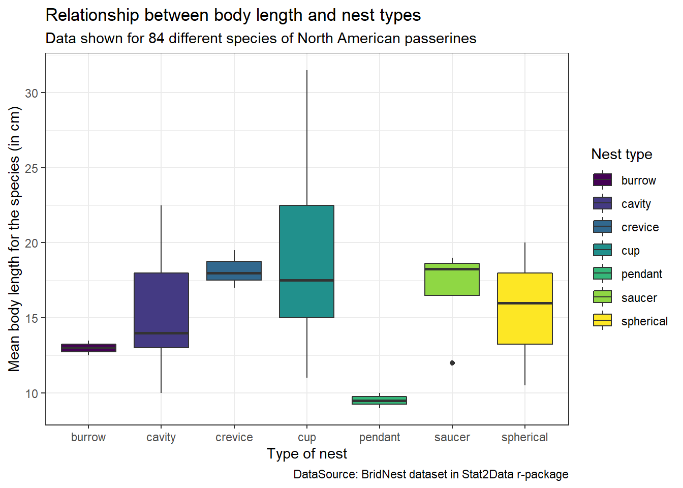

magma

Show the code

library(Stat2Data)
library(viridis)
data("BirdNest")

ggplot(BirdNest, aes(Nesttype, Length, fill = Nesttype)) + geom_boxplot() + 
  labs(x= "Type of nest", y= "Mean body length for the species (in cm)",
       fill= "Nest type", title= "Relationship between body length and nest types",
       subtitle = "Data shown for 84 different species of North American passerines",
       caption= "DataSource: BridNest dataset in Stat2Data r-package") +
  theme_bw() + scale_fill_viridis(discrete = TRUE, option = "magma")

plasma

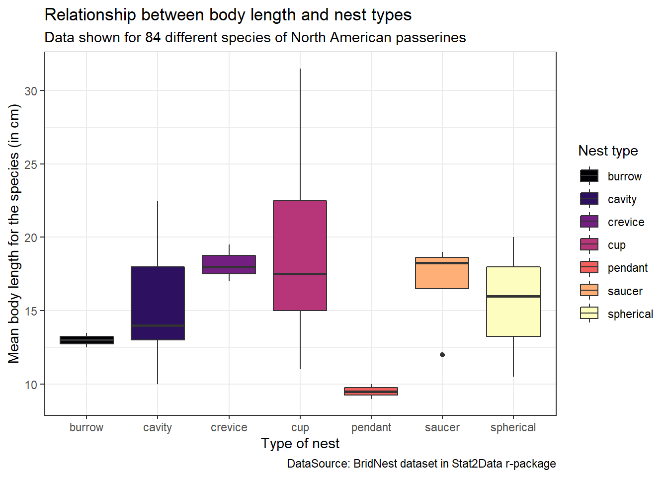
Show the code

library(Stat2Data)
library(viridis)
data("BirdNest")

ggplot(BirdNest, aes(Nesttype, Length, fill = Nesttype)) + geom_boxplot() + 
  labs(x= "Type of nest", y= "Mean body length for the species (in cm)",
       fill= "Nest type", title= "Relationship between body length and nest types",
       subtitle = "Data shown for 84 different species of North American passerines",
       caption= "DataSource: BridNest dataset in Stat2Data r-package") +
  theme_bw() + scale_fill_viridis(discrete = TRUE, option = "plasma")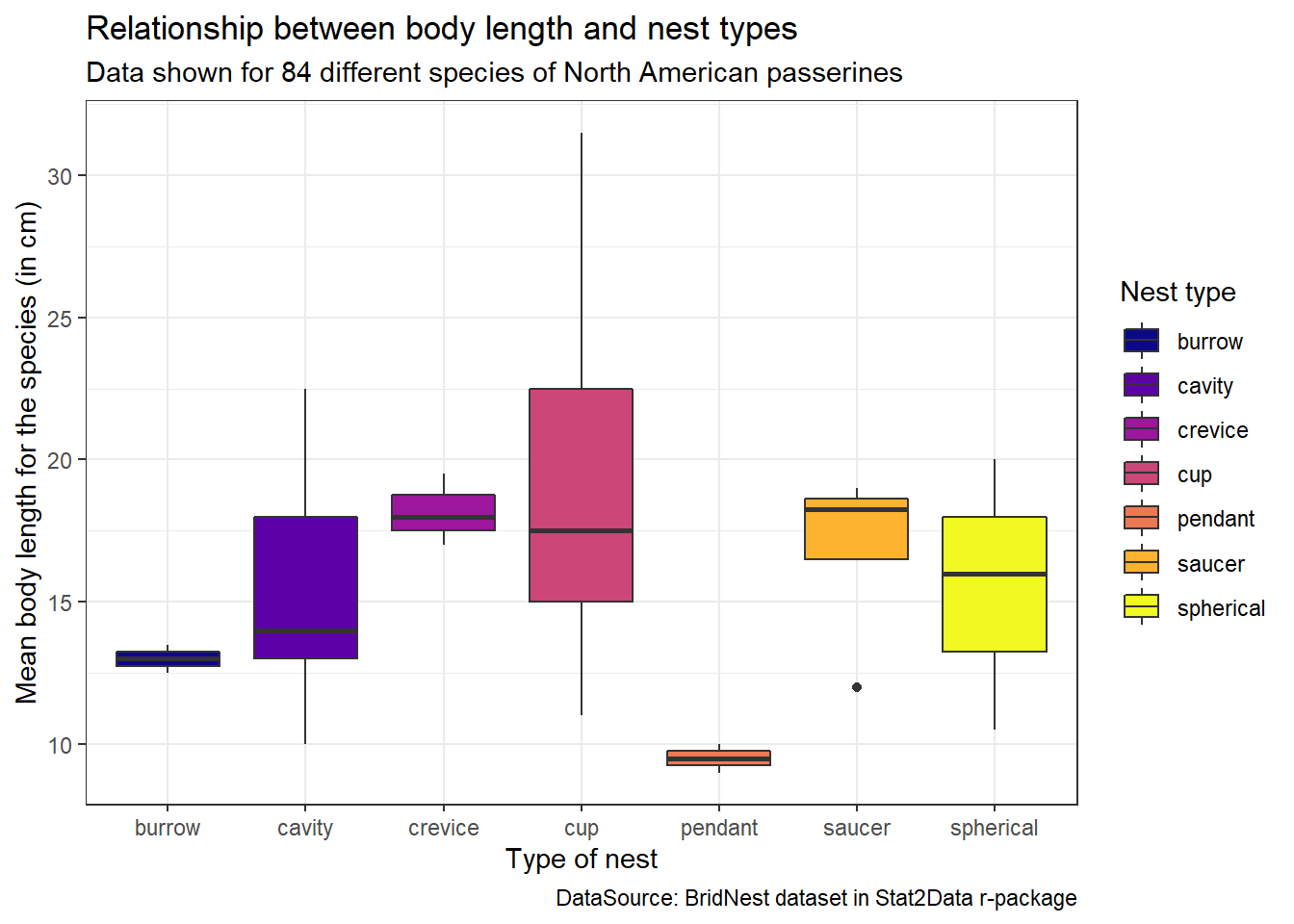

inferno

Show the code

library(Stat2Data)
library(viridis)
data("BirdNest")

ggplot(BirdNest, aes(Nesttype, Length, fill = Nesttype)) + geom_boxplot() + 
  labs(x= "Type of nest", y= "Mean body length for the species (in cm)",
       fill= "Nest type", title= "Relationship between body length and nest types",
       subtitle = "Data shown for 84 different species of North American passerines",
       caption= "DataSource: BridNest dataset in Stat2Data r-package") +
  theme_bw() + scale_fill_viridis(discrete = TRUE, option = "inferno")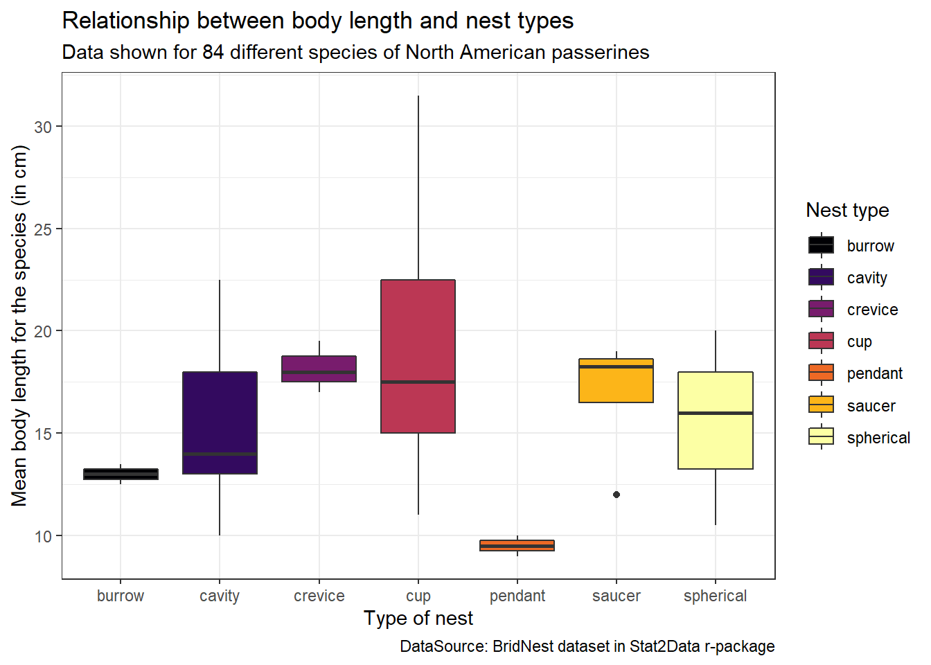

cividis

Show the code

library(Stat2Data)
library(viridis)
data("BirdNest")

ggplot(BirdNest, aes(Nesttype, Length, fill = Nesttype)) + geom_boxplot() + 
  labs(x= "Type of nest", y= "Mean body length for the species (in cm)",
       fill= "Nest type", title= "Relationship between body length and nest types",
       subtitle = "Data shown for 84 different species of North American passerines",
       caption= "DataSource: BridNest dataset in Stat2Data r-package") +
  theme_bw() + scale_fill_viridis(discrete = TRUE, option = "cividis")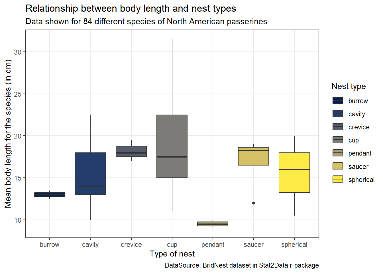

mako

Show the code

library(Stat2Data)
library(viridis)
data("BirdNest")

ggplot(BirdNest, aes(Nesttype, Length, fill = Nesttype)) + geom_boxplot() + 
  labs(x= "Type of nest", y= "Mean body length for the species (in cm)",
       fill= "Nest type", title= "Relationship between body length and nest types",
       subtitle = "Data shown for 84 different species of North American passerines",
       caption= "DataSource: BridNest dataset in Stat2Data r-package") +
  theme_bw() + scale_fill_viridis(discrete = TRUE, option = "mako")

rocket

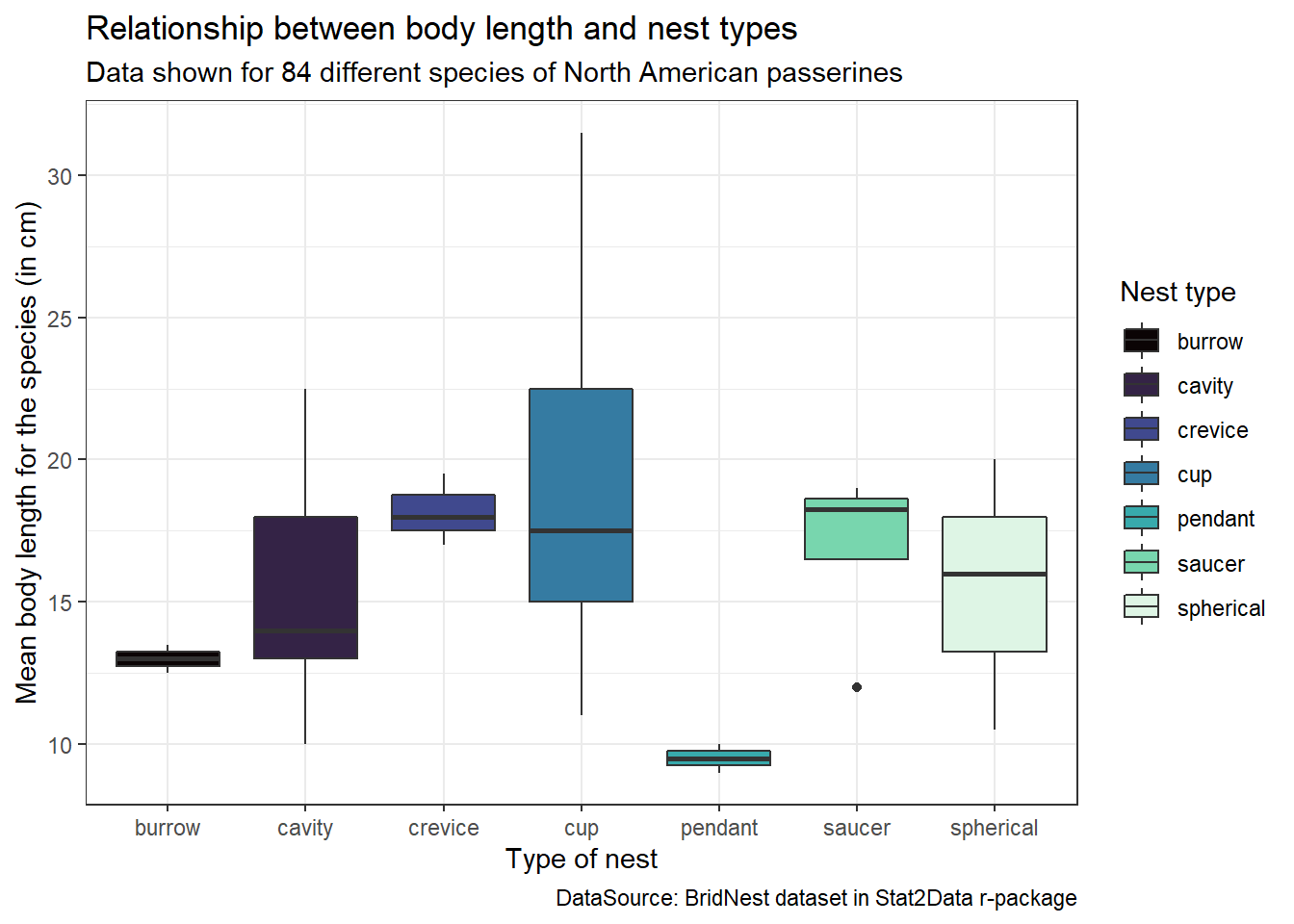
Show the code

library(Stat2Data)
library(viridis)
data("BirdNest")

ggplot(BirdNest, aes(Nesttype, Length, fill = Nesttype)) + geom_boxplot() + 
  labs(x= "Type of nest", y= "Mean body length for the species (in cm)",
       fill= "Nest type", title= "Relationship between body length and nest types",
       subtitle = "Data shown for 84 different species of North American passerines",
       caption= "DataSource: BridNest dataset in Stat2Data r-package") +
  theme_bw() + scale_fill_viridis(discrete = TRUE, option = "rocket")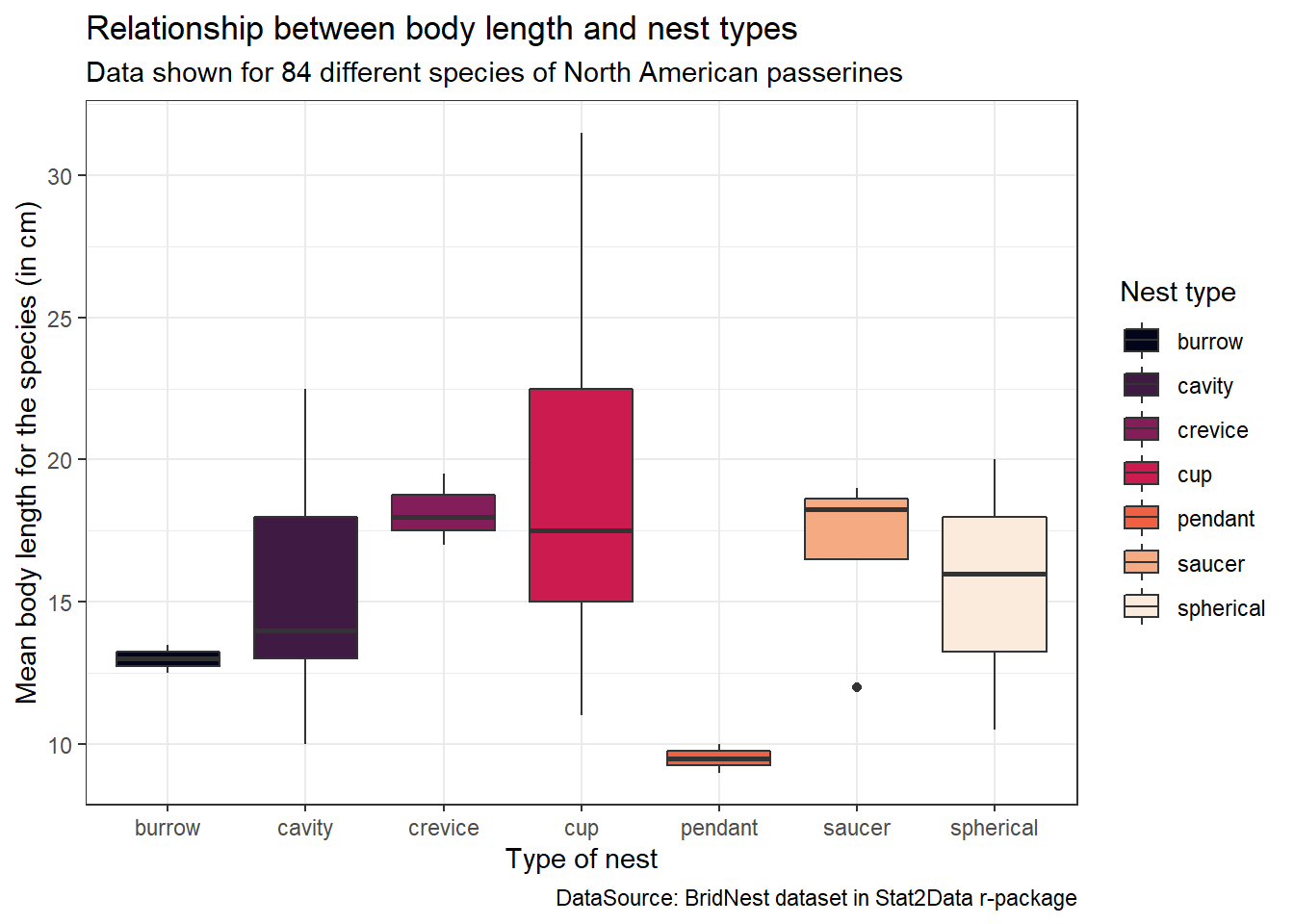

turbo

Show the code

library(Stat2Data)
library(viridis)
data("BirdNest")

ggplot(BirdNest, aes(Nesttype, Length, fill = Nesttype)) + geom_boxplot() + 
  labs(x= "Type of nest", y= "Mean body length for the species (in cm)",
       fill= "Nest type", title= "Relationship between body length and nest types",
       subtitle = "Data shown for 84 different species of North American passerines",
       caption= "DataSource: BridNest dataset in Stat2Data r-package") +
  theme_bw() + scale_fill_viridis(discrete = TRUE, option = "turbo")

3.2 wesanderson package

If you like your colours distinctive and narrative, just like how American film-maker Mr. Wes Anderson would like it, then try the {wesanderson} package. Relive the The Grand Budapest Hotel moments through your graphs. The {wesanderson} package was developed by Karthik Ram. There are a total of 19 colour palettes present in this package. We will see a subset of them. All colour scales in this package are available here. The name of the tab denotes the colour scale used. The data used in this plot is the penguin dataset present in the package {palmerpenguins}.

#install and load wesanderson and palmerpenguins package
install.packages("wesanderson")
install.packages("palmerpenguins")
library(wesanderson)
library(palmerpenguins)
data("penguins") #load the penguins dataset

GrandBudapest1

Show the code

library(wesanderson)
library(palmerpenguins)
data("penguins")

ggplot(data = penguins, aes(x = species, y = body_mass_g, fill = species)) + 
  labs(x= "Species", y= "Body mass (g)",
       fill= "Nest type", title= "Body mass in three diferent species of penguins",
       subtitle = "Penguins observed on islands near Palmer Station, Antarctica",
       caption= "DataSource: penguins dataset in palmerpenguins r-package") + geom_boxplot() + 
  theme_bw() + scale_fill_manual(values = wes_palette("GrandBudapest1", n = 3))

BottleRocket2

Show the code

library(wesanderson)
library(palmerpenguins)
data("penguins")

ggplot(data = penguins, aes(x = species, y = body_mass_g, fill = species)) + 
  labs(x= "Species", y= "Body mass (g)",
       fill= "Nest type", title= "Body mass in three diferent species of penguins",
       subtitle = "Penguins observed on islands near Palmer Station, Antarctica",
       caption= "DataSource: penguins dataset in palmerpenguins r-package") + geom_boxplot() + 
  theme_bw() + scale_fill_manual(values = wes_palette("BottleRocket2", n = 3))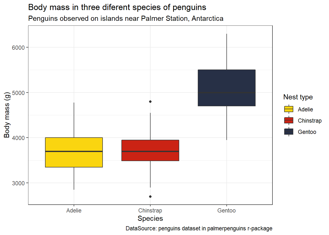

Rushmore1

Show the code

library(wesanderson)
library(palmerpenguins)
data("penguins")

ggplot(data = penguins, aes(x = species, y = body_mass_g, fill = species)) + 
  labs(x= "Species", y= "Body mass (g)",
       fill= "Nest type", title= "Body mass in three diferent species of penguins",
       subtitle = "Penguins observed on islands near Palmer Station, Antarctica",
       caption= "DataSource: penguins dataset in palmerpenguins r-package") + geom_boxplot() + 
  theme_bw() + scale_fill_manual(values = wes_palette("Rushmore1", n = 3))

Royal1

Show the code

library(wesanderson)
library(palmerpenguins)
data("penguins")

ggplot(data = penguins, aes(x = species, y = body_mass_g, fill = species)) + 
  labs(x= "Species", y= "Body mass (g)",
       fill= "Nest type", title= "Body mass in three diferent species of penguins",
       subtitle = "Penguins observed on islands near Palmer Station, Antarctica",
       caption= "DataSource: penguins dataset in palmerpenguins r-package") + geom_boxplot() + 
  theme_bw() + scale_fill_manual(values = wes_palette("Royal1", n = 3))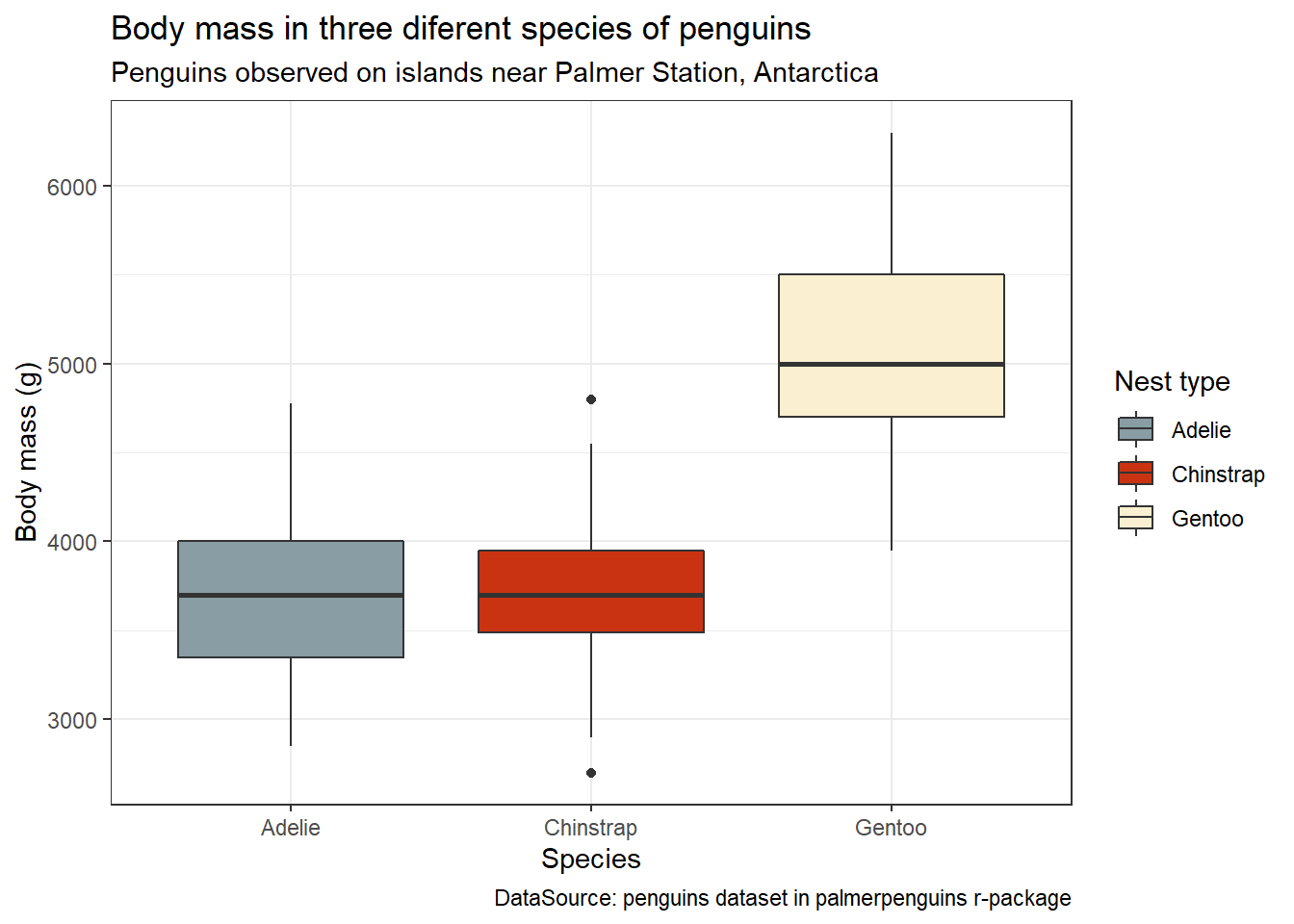

Zissou1

Show the code

library(wesanderson)
library(palmerpenguins)
data("penguins")

ggplot(data = penguins, aes(x = species, y = body_mass_g, fill = species)) + 
  labs(x= "Species", y= "Body mass (g)",
       fill= "Nest type", title= "Body mass in three diferent species of penguins",
       subtitle = "Penguins observed on islands near Palmer Station, Antarctica",
       caption= "DataSource: penguins dataset in palmerpenguins r-package") + geom_boxplot() + 
  theme_bw() + scale_fill_manual(values = wes_palette("Zissou1", n = 3))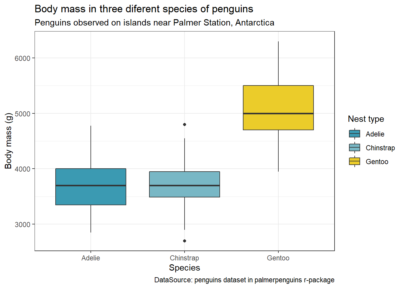

Darjeeling2

Show the code

library(wesanderson)
library(palmerpenguins)
data("penguins")

ggplot(data = penguins, aes(x = species, y = body_mass_g, fill = species)) + 
  labs(x= "Species", y= "Body mass (g)",
       fill= "Nest type", title= "Body mass in three diferent species of penguins",
       subtitle = "Penguins observed on islands near Palmer Station, Antarctica",
       caption= "DataSource: penguins dataset in palmerpenguins r-package") + geom_boxplot() + 
  theme_bw() + scale_fill_manual(values = wes_palette("Darjeeling2", n = 3))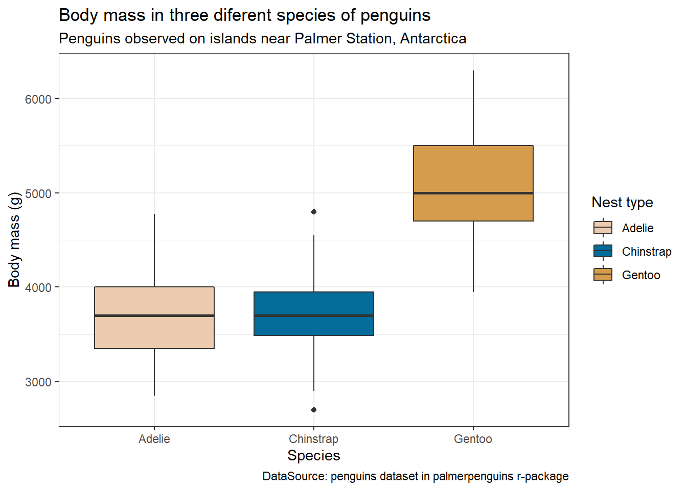

IsleofDogs1

Show the code

library(wesanderson)
library(palmerpenguins)
data("penguins")

ggplot(data = penguins, aes(x = species, y = body_mass_g, fill = species)) + 
  labs(x= "Species", y= "Body mass (g)",
       fill= "Nest type", title= "Body mass in three diferent species of penguins",
       subtitle = "Penguins observed on islands near Palmer Station, Antarctica",
       caption= "DataSource: penguins dataset in palmerpenguins r-package") + geom_boxplot() + 
  theme_bw() + scale_fill_manual(values = wes_palette("IsleofDogs1", n = 3))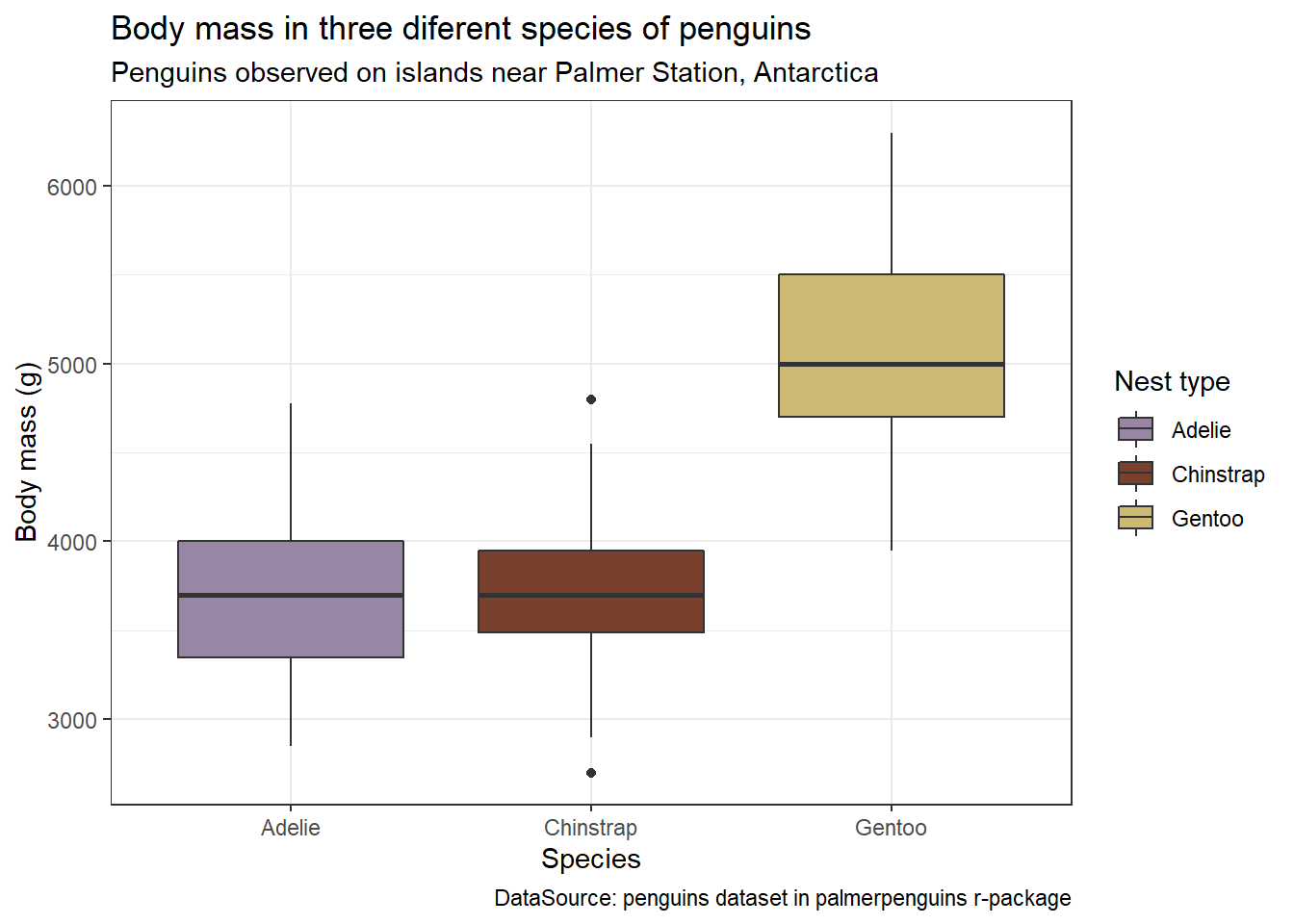

3.3 ggsci package

If you want high-quality colour palettes reflecting scientific journal styles then you can try the {ggsci} package. The {ggsci} package was developed by Dr. Nan Xiao and Dr. Miaozhu Li. All colour scales in this package are available in package webpage. The name of the tab denotes the colour scale used.

# load ggsci package
install.packages("ggsci")
library(ggsci)

npg

Show the code

library(ggsci)
library(Stat2Data)
data("BirdNest")

ggplot(BirdNest, aes(Nesttype, Length, fill = Nesttype)) + geom_boxplot() + 
  labs(x= "Type of nest", y= "Mean body length for the species (in cm)",
       fill= "Nest type", title= "Relationship between body length and nest types",
       subtitle = "Data shown for 84 different species of North American passerines",
       caption= "DataSource: BridNest dataset in Stat2Data r-package") +
  theme_bw() + scale_fill_npg()

aaas

Show the code

library(ggsci)
library(Stat2Data)
data("BirdNest")

ggplot(BirdNest, aes(Nesttype, Length, fill = Nesttype)) + geom_boxplot() + 
  labs(x= "Type of nest", y= "Mean body length for the species (in cm)",
       fill= "Nest type", title= "Relationship between body length and nest types",
       subtitle = "Data shown for 84 different species of North American passerines",
       caption= "DataSource: BridNest dataset in Stat2Data r-package") +
  theme_bw() + scale_fill_aaas()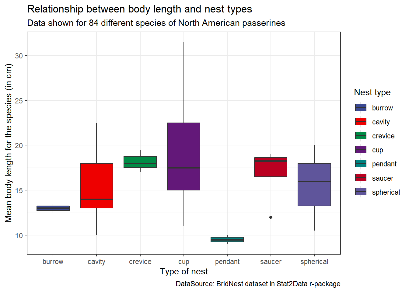

nejm

Show the code

library(ggsci)
library(Stat2Data)
data("BirdNest")

ggplot(BirdNest, aes(Nesttype, Length, fill = Nesttype)) + geom_boxplot() + 
  labs(x= "Type of nest", y= "Mean body length for the species (in cm)",
       fill= "Nest type", title= "Relationship between body length and nest types",
       subtitle = "Data shown for 84 different species of North American passerines",
       caption= "DataSource: BridNest dataset in Stat2Data r-package") +
  theme_bw() + scale_fill_nejm()

lancet

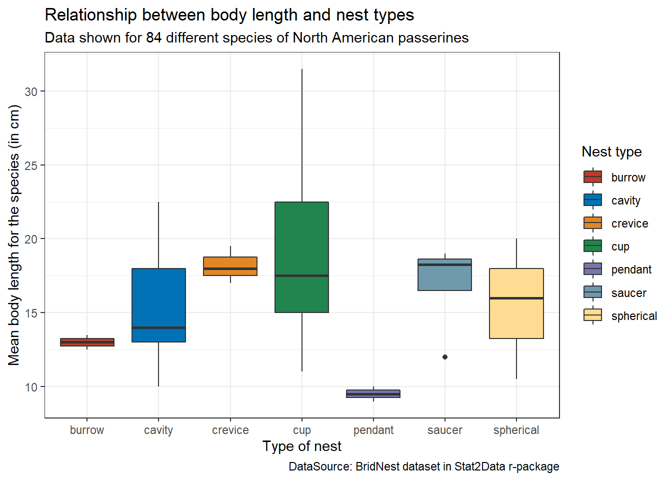
Show the code

library(ggsci)
library(Stat2Data)
data("BirdNest")

ggplot(BirdNest, aes(Nesttype, Length, fill = Nesttype)) + geom_boxplot() + 
  labs(x= "Type of nest", y= "Mean body length for the species (in cm)",
       fill= "Nest type", title= "Relationship between body length and nest types",
       subtitle = "Data shown for 84 different species of North American passerines",
       caption= "DataSource: BridNest dataset in Stat2Data r-package") +
  theme_bw() + scale_fill_lancet()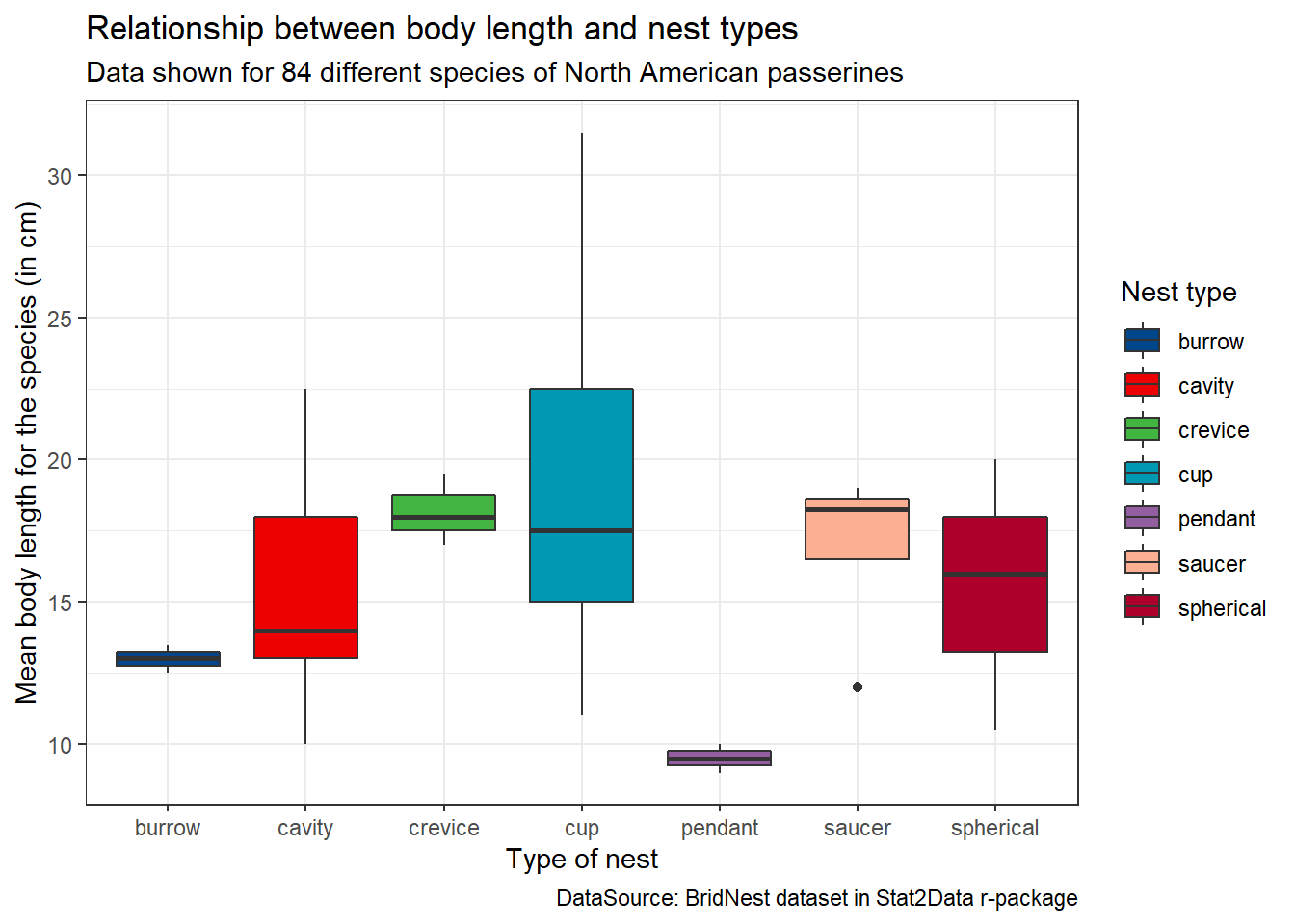

jama

Show the code

library(ggsci)
library(Stat2Data)
data("BirdNest")

ggplot(BirdNest, aes(Nesttype, Length, fill = Nesttype)) + geom_boxplot() + 
  labs(x= "Type of nest", y= "Mean body length for the species (in cm)",
       fill= "Nest type", title= "Relationship between body length and nest types",
       subtitle = "Data shown for 84 different species of North American passerines",
       caption= "DataSource: BridNest dataset in Stat2Data r-package") +
  theme_bw() + scale_fill_jama()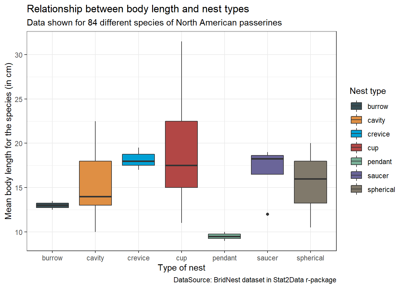

jco

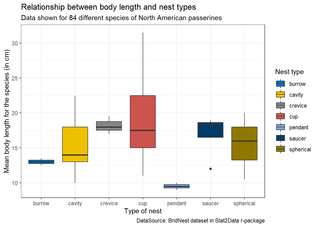
Show the code

library(ggsci)
library(Stat2Data)
data("BirdNest")

ggplot(BirdNest, aes(Nesttype, Length, fill = Nesttype)) + geom_boxplot() + 
  labs(x= "Type of nest", y= "Mean body length for the species (in cm)",
       fill= "Nest type", title= "Relationship between body length and nest types",
       subtitle = "Data shown for 84 different species of North American passerines",
       caption= "DataSource: BridNest dataset in Stat2Data r-package") +
  theme_bw() + scale_fill_jco()

ucscgb

Show the code

library(ggsci)
library(Stat2Data)
data("BirdNest")

ggplot(BirdNest, aes(Nesttype, Length, fill = Nesttype)) + geom_boxplot() + 
  labs(x= "Type of nest", y= "Mean body length for the species (in cm)",
       fill= "Nest type", title= "Relationship between body length and nest types",
       subtitle = "Data shown for 84 different species of North American passerines",
       caption= "DataSource: BridNest dataset in Stat2Data r-package") +
  theme_bw() + scale_fill_ucscgb()

d3

Show the code

library(ggsci)
library(Stat2Data)
data("BirdNest")

ggplot(BirdNest, aes(Nesttype, Length, fill = Nesttype)) + geom_boxplot() + 
  labs(x= "Type of nest", y= "Mean body length for the species (in cm)",
       fill= "Nest type", title= "Relationship between body length and nest types",
       subtitle = "Data shown for 84 different species of North American passerines",
       caption= "DataSource: BridNest dataset in Stat2Data r-package") +
  theme_bw() + scale_fill_d3(palette = "category10")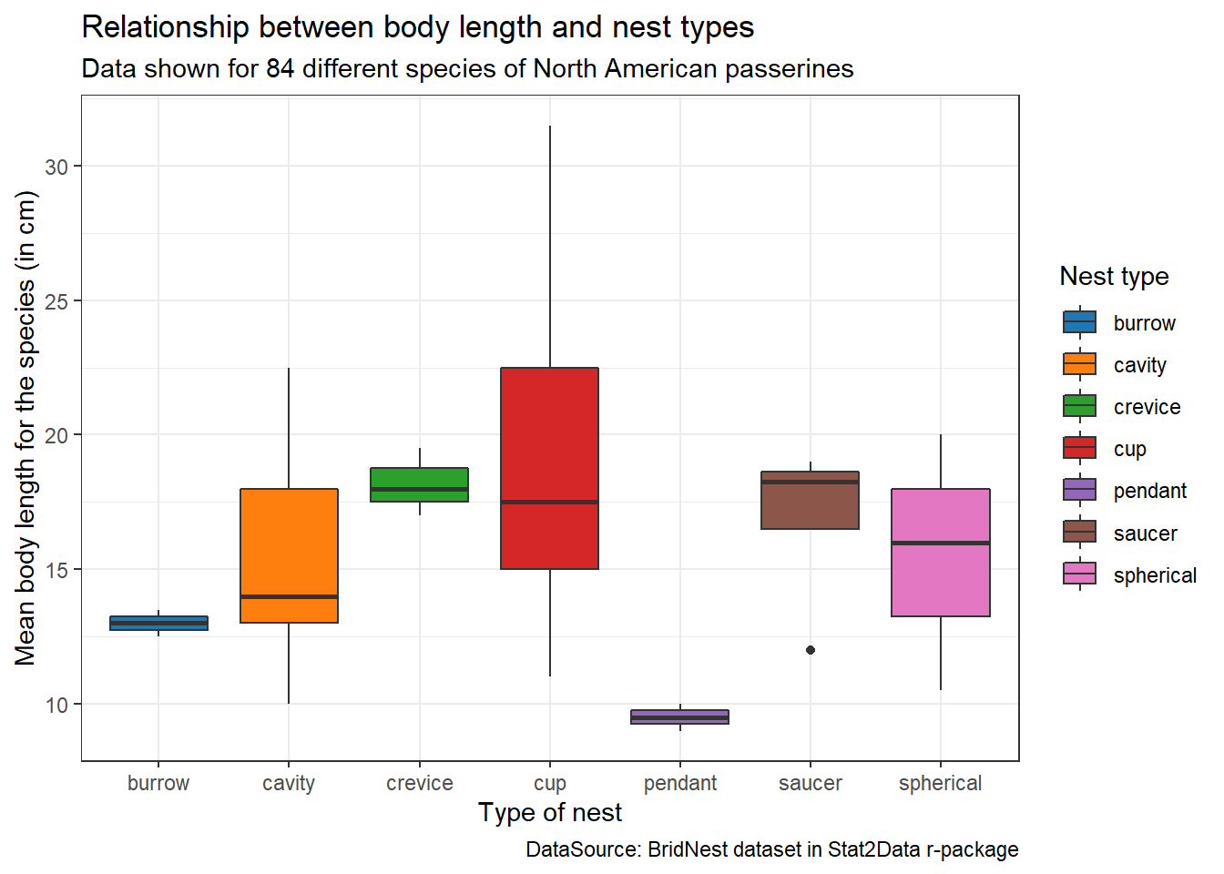

locuszoom

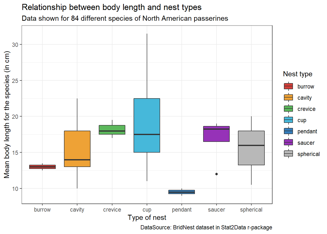
Show the code

library(ggsci)
library(Stat2Data)
data("BirdNest")

ggplot(BirdNest, aes(Nesttype, Length, fill = Nesttype)) + geom_boxplot() + 
  labs(x= "Type of nest", y= "Mean body length for the species (in cm)",
       fill= "Nest type", title= "Relationship between body length and nest types",
       subtitle = "Data shown for 84 different species of North American passerines",
       caption= "DataSource: BridNest dataset in Stat2Data r-package") +
  theme_bw() + scale_fill_locuszoom()

igv

Show the code

library(ggsci)
library(Stat2Data)
data("BirdNest")

ggplot(BirdNest, aes(Nesttype, Length, fill = Nesttype)) + geom_boxplot() + 
  labs(x= "Type of nest", y= "Mean body length for the species (in cm)",
       fill= "Nest type", title= "Relationship between body length and nest types",
       subtitle = "Data shown for 84 different species of North American passerines",
       caption= "DataSource: BridNest dataset in Stat2Data r-package") +
  theme_bw() + scale_fill_igv()

uchicago

Show the code

library(ggsci)
library(Stat2Data)
data("BirdNest")

ggplot(BirdNest, aes(Nesttype, Length, fill = Nesttype)) + geom_boxplot() + 
  labs(x= "Type of nest", y= "Mean body length for the species (in cm)",
       fill= "Nest type", title= "Relationship between body length and nest types",
       subtitle = "Data shown for 84 different species of North American passerines",
       caption= "DataSource: BridNest dataset in Stat2Data r-package") +
  theme_bw() + scale_fill_uchicago()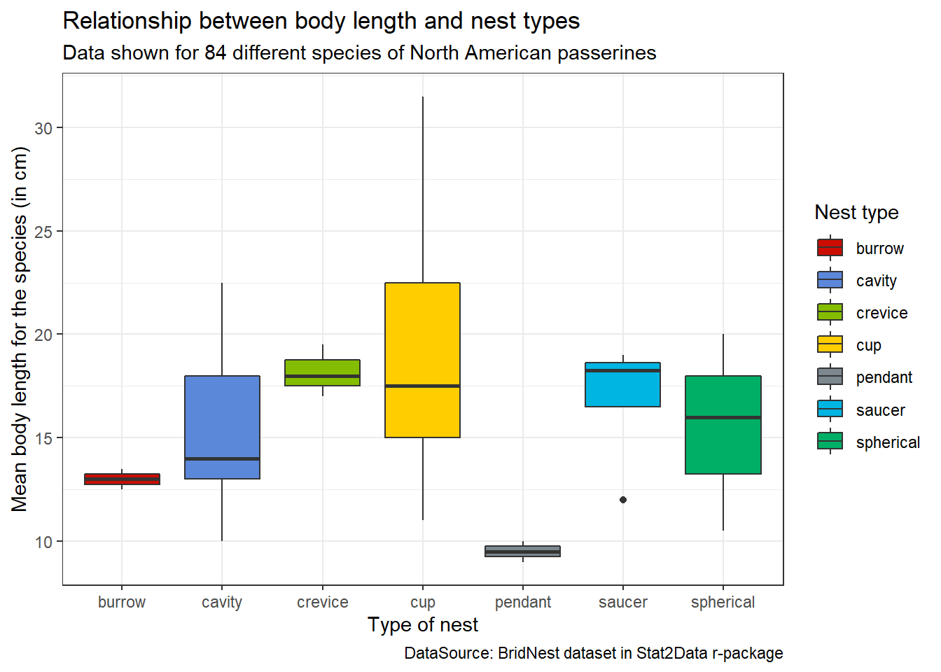

startrek

Show the code

library(ggsci)
library(Stat2Data)
data("BirdNest")

ggplot(BirdNest, aes(Nesttype, Length, fill = Nesttype)) + geom_boxplot() + 
  labs(x= "Type of nest", y= "Mean body length for the species (in cm)",
       fill= "Nest type", title= "Relationship between body length and nest types",
       subtitle = "Data shown for 84 different species of North American passerines",
       caption= "DataSource: BridNest dataset in Stat2Data r-package") +
  theme_bw() + scale_fill_startrek()

tron

Show the code

library(ggsci)
library(Stat2Data)
data("BirdNest")

ggplot(BirdNest, aes(Nesttype, Length, fill = Nesttype)) + geom_boxplot() + 
  labs(x= "Type of nest", y= "Mean body length for the species (in cm)",
       fill= "Nest type", title= "Relationship between body length and nest types",
       subtitle = "Data shown for 84 different species of North American passerines",
       caption= "DataSource: BridNest dataset in Stat2Data r-package") +
  theme_bw() + scale_fill_tron()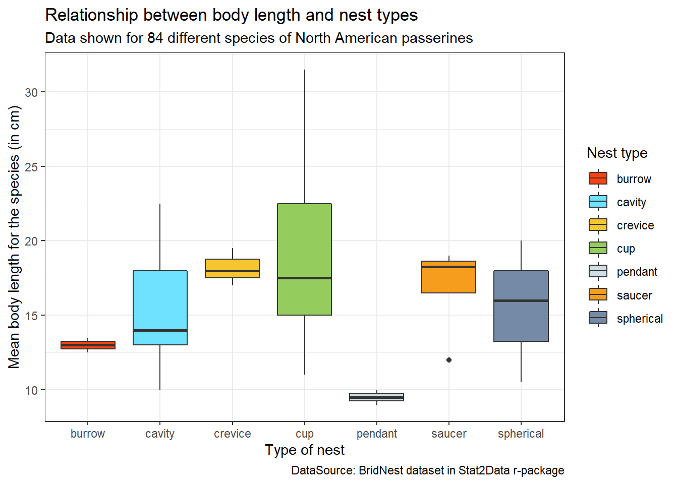

futurama

Show the code

library(ggsci)
library(Stat2Data)
data("BirdNest")

ggplot(BirdNest, aes(Nesttype, Length, fill = Nesttype)) + geom_boxplot() + 
  labs(x= "Type of nest", y= "Mean body length for the species (in cm)",
       fill= "Nest type", title= "Relationship between body length and nest types",
       subtitle = "Data shown for 84 different species of North American passerines",
       caption= "DataSource: BridNest dataset in Stat2Data r-package") +
  theme_bw() + scale_fill_futurama()

rickandmorty

Show the code

library(ggsci)
library(Stat2Data)
data("BirdNest")

ggplot(BirdNest, aes(Nesttype, Length, fill = Nesttype)) + geom_boxplot() + 
  labs(x= "Type of nest", y= "Mean body length for the species (in cm)",
       fill= "Nest type", title= "Relationship between body length and nest types",
       subtitle = "Data shown for 84 different species of North American passerines",
       caption= "DataSource: BridNest dataset in Stat2Data r-package") +
  theme_bw() + scale_fill_rickandmorty()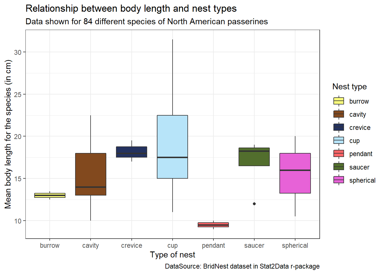

simpsons

Show the code

library(ggsci)
library(Stat2Data)
data("BirdNest")

ggplot(BirdNest, aes(Nesttype, Length, fill = Nesttype)) + geom_boxplot() + 
  labs(x= "Type of nest", y= "Mean body length for the species (in cm)",
       fill= "Nest type", title= "Relationship between body length and nest types",
       subtitle = "Data shown for 84 different species of North American passerines",
       caption= "DataSource: BridNest dataset in Stat2Data r-package") +
  theme_bw() + scale_fill_simpsons()

4 Customizing the theme()

A ggplot theme is made up of different elements and it’s functions. For e.g. plot.title() element allows you to modify the title of the graph using the element function element_text(). In this way, we can change the font size, font family, text colour etc. of the title of the plot. So let us begin customising our graph. We will be reusing the BirdNest dataset for the graphs.

4.1 Customizing text elements using element_text()

All text elements can be customized using the element function element_text(). The syntax for element_text() is as follows

element_text(
  family = NULL, #insert family font name, e.g. "Times"
  face = NULL,  #font face ("plain", "italic", "bold", "bold.italic")
  colour = NULL, #either from colours() or hex code inside ""
  size = NULL, #text size (in pts)
  hjust = NULL, #horizontal justification values 0 or 1
  vjust = NULL, #vertical justification values 0 or 1
  angle = NULL, #angle in degrees
  lineheight = NULL, #distance between text and axis line
  color = NULL, #same function as colour
  margin = NULL,
  debug = NULL,
  inherit.blank = FALSE
)

We can modify each of these parameters to improve our plots as shown below in ‘before’ and ‘after’ the changes are made.

Before

Show the code

library(ggplot2)
library(Stat2Data)
data("BirdNest")

p <- ggplot(BirdNest, aes(No.eggs, Totcare, colour = Nesttype)) + geom_point() +
    labs(x= "Number of eggs", y= "Total care time (days)",
       title= "Relationship between number of eggs and total care time",
       subtitle = "Data shown for 84 different species of North American passerines",
       caption= "DataSource: BridNest dataset in Stat2Data r-package",
       colour = "Nest type")
p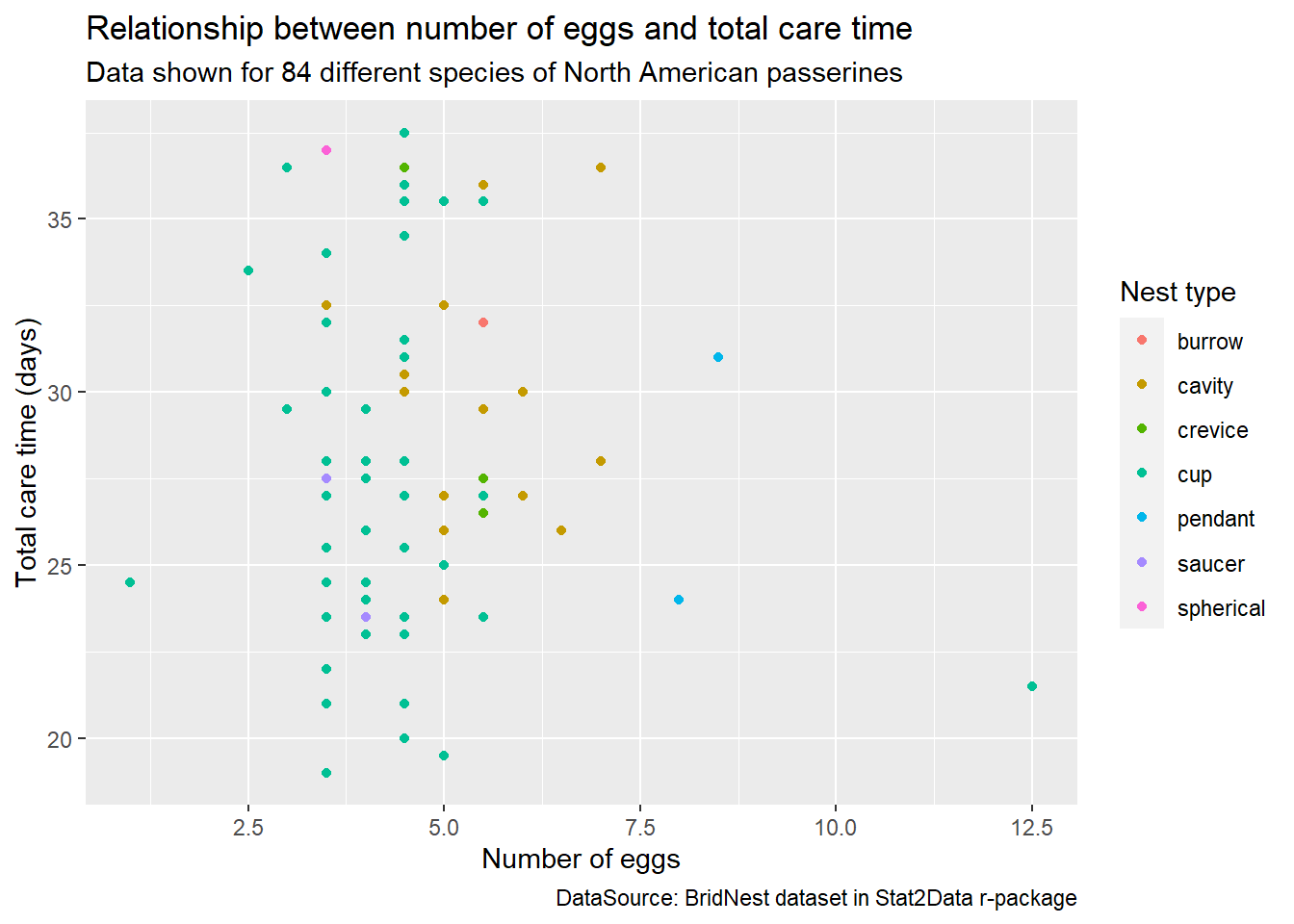

After

Show the code

library(ggplot2)
library(Stat2Data)
data("BirdNest")

p <- ggplot(BirdNest, aes(No.eggs, Totcare, colour = Nesttype)) + geom_point() +
    labs(x= "Number of eggs", y= "Total care time (days)",
       title= "Relationship between number of eggs and total care time",
       subtitle = "Data shown for 84 different species of North American passerines",
       caption= "DataSource: BridNest dataset in Stat2Data r-package",
       colour = "Nest type")

#customizing text elements
p + theme(plot.title=element_text(size = 15,family = "Comic Sans MS",colour = "darkred",face = "bold"),
          plot.subtitle=element_text(size = 10,family = "Courier",colour= "blue",face= "italic"),
          plot.caption = element_text(size = 8,family = "Times",colour= "green",face="bold.italic", hjust=0),
          axis.text.x= element_text(size = 6,colour = "magenta", angle=20),
          axis.text.y= element_text(size = 6,colour = "darkblue", angle=30),
          axis.title.x = element_text(colour = "orchid"),
          axis.title.y = element_text(colour = "sienna"),
          legend.text = element_text(size = 8,colour = "darkgreen"),
          legend.title = element_text(size = 10,colour = "lightblue",face = "bold"))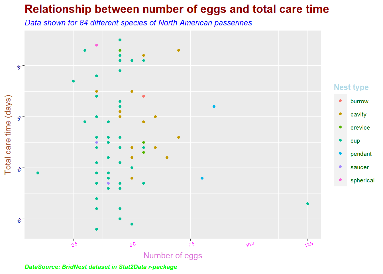

4.2 Customizing line elements using element_line()

Line elements include axes, grid lines, borders of the graph etc. All line elements can be customized using the element function element_line(). The syntax for element_line() is as follows

element_line(
  colour = NULL, #either from colours() or hex code inside ""
  size = NULL, #line size in mm units
  linetype = NULL, # eg: dashed, dotted etc 
  lineend = NULL, #line end style (round, butt, square)
  color = NULL, #same function as colour
  arrow = NULL, #arrow specification
  inherit.blank = FALSE
)

Before

Show the code

library(ggplot2)
library(Stat2Data)
data("BirdNest")

p <- ggplot(BirdNest, aes(Nesttype, Length, fill = Nesttype)) + geom_boxplot() + 
  labs(x= "Type of nest", y= "Mean body length for the species (in cm)",
       fill= "Nest type", title= "Relationship between body length and nest types",
       subtitle = "Data shown for 84 different species of North American passerines",
       caption= "DataSource: BridNest dataset in Stat2Data r-package")
p

After

Show the code

library(ggplot2)
library(Stat2Data)
data("BirdNest")

p <- ggplot(BirdNest, aes(Nesttype, Length, fill = Nesttype)) + geom_boxplot() + 
  labs(x= "Type of nest", y= "Mean body length for the species (in cm)",
       fill= "Nest type", title= "Relationship between body length and nest types",
       subtitle = "Data shown for 84 different species of North American passerines",
       caption= "DataSource: BridNest dataset in Stat2Data r-package")

#customizing line elements
p + theme(panel.grid.major = element_line(colour = "red", size = 0.8, linetype = "dashed"),
          panel.grid.minor = element_line(colour = "blue",linetype = "twodash"),
          axis.line.x = element_line(colour = "darkred", arrow = arrow()),
          axis.line.y = element_line(colour = "darkblue"),
          axis.ticks = element_line(size = 5, colour = "yellow"),
          axis.ticks.length.y=unit(0.5, "cm")) #ticks positioned 0.5cm away from y axis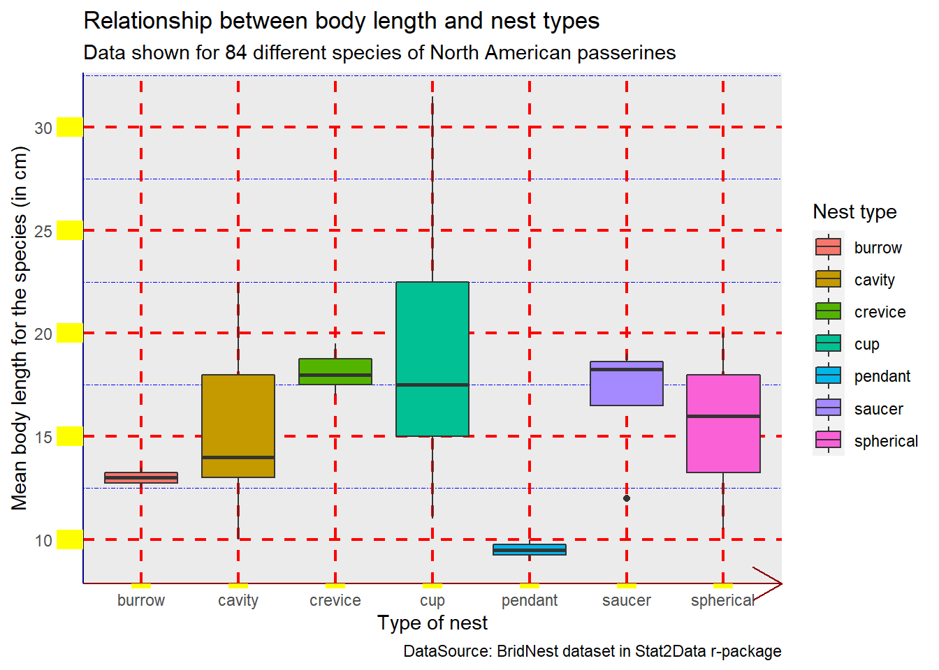

4.3 Customizing background elements using element_rect()

Background elements include plot, panel and legend backgrounds and their margins. All background elements can be customized using the element function element_rect(). The syntax for element_rect() is as follows

element_rect(
  fill = NULL, #fills colour
  colour = NULL, #colours the border
  size = NULL, #changes border size in mm units
  linetype = NULL, #changes border linetype
  color = NULL,
  inherit.blank = FALSE
)

Before

Show the code

library(ggplot2)
library(Stat2Data)
data("BirdNest")

p <- ggplot(BirdNest, aes(Nesttype, Length, fill = Nesttype)) + geom_boxplot() + 
  labs(x= "Type of nest", y= "Mean body length for the species (in cm)",
       fill= "Nest type", title= "Relationship between body length and nest types",
       subtitle = "Data shown for 84 different species of North American passerines",
       caption= "DataSource: BridNest dataset in Stat2Data r-package")
p

After

Show the code

library(ggplot2)
library(Stat2Data)
data("BirdNest")

p <- ggplot(BirdNest, aes(Nesttype, Length, fill = Nesttype)) + geom_boxplot() + 
  labs(x= "Type of nest", y= "Mean body length for the species (in cm)",
       fill= "Nest type", title= "Relationship between body length and nest types",
       subtitle = "Data shown for 84 different species of North American passerines",
       caption= "DataSource: BridNest dataset in Stat2Data r-package")

#customizing line elements
p + theme(plot.background = element_rect(size = 5, colour = "red", fill = "lightblue"),
          panel.background = element_rect(size = 3, colour = "blue", fill = "lightyellow", linetype = "dotted"),
          legend.key = element_rect(fill = "lightgreen"),
          legend.background = element_rect(fill = "grey"),
          legend.key.size = unit(0.75, "cm"))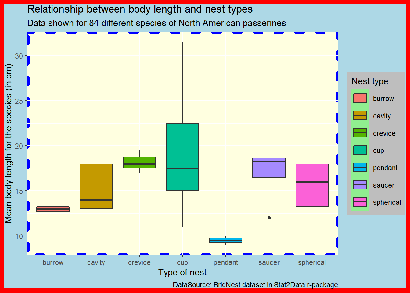

5 Summary

I hope you are now able to customize the theme of a graph with ease. In this chapter, we learned about different theme elements and how to customize them. We also saw different packages in R which featured ready to use themes. We learned about colour palettes and got introduced to the popular colour packages available R. With that being said, always make sure that your graphs are colour-blind friendly.

6 References

1. H. Wickham. ggplot2: Elegant Graphics for Data Analysis. Springer-Verlag New York, 2016. Read more about ggplot2 here. You can also look at the cheat sheet for all the syntax used in ggplot2. Also check this out.

2. Ann Cannon, George Cobb, Bradley Hartlaub, Julie Legler, Robin Lock, Thomas Moore, Allan Rossman and Jeffrey Witmer (2019). Stat2Data: Datasets for Stat2. R package version 2.0.0. https://CRAN.R-project.org/package=Stat2Data

3. Horst AM, Hill AP, Gorman KB (2020). palmerpenguins: Palmer Archipelago (Antarctica) penguin data. R package version 0.1.0. https://allisonhorst.github.io/palmerpenguins/

4. Jeffrey B. Arnold (2021). ggthemes: Extra Themes, Scales and Geoms for ‘ggplot2’. R package version 4.2.4. https://CRAN.R-project.org/package=ggthemes

5. Simon Garnier, Noam Ross, Robert Rudis, Antônio P. Camargo, Marco Sciaini, and Cédric Scherer (2021). Rvision - Colorblind-Friendly Color Maps for R. R package version 0.6.2. You can read more here.

6. Karthik Ram and Hadley Wickham (2018). wesanderson: A Wes Anderson Palette Generator. R package version 0.3.6. https://CRAN.R-project.org/package=wesanderson

7. Nan Xiao (2018). ggsci: Scientific Journal and Sci-Fi Themed Color Palettes for ‘ggplot2’. R package version 2.9. https://CRAN.R-project.org/package=ggsci

Reuse

Citation

BibTeX citation:

@online{johnson2021,
  author = {Johnson, Jewel},
  title = {Chapter 3: {Even} More Customizations in Ggplot2},
  date = {2021-12-09},
  url = {https://sciquest.netlify.app//tutorials/data_viz/ggplot_3.html},
  langid = {en}
}

For attribution, please cite this work as:

Johnson, Jewel. 2021. “Chapter 3: Even More Customizations in Ggplot2.” December 9, 2021. https://sciquest.netlify.app//tutorials/data_viz/ggplot_3.html.